

Sentinel-1 RTC Stack Processor
The radiometric terrain correction (RTC) stacking tool facilitates time-series analysis of such phenomena as flooding events, deforestation, or glacier retreat.
This tool creates a stack from a set of Sentinel-1 RTC products produced on the ASF HyP3 system. It also works for a co-registered set of PALSAR RTC products. In fact the tool can accept any UTM projected co-registered set of images.
The stack tool allows the user to perform sub-setting, resampling, grouping, filtering, and culling on the stack. The final products are a stack of processed geotiffs and an animated GIF of the stack.
For installation instructions and to download the code, procS1StackRTC.py, please visit our GitHub repo and select “RTC Time Series Generation Using HYP3 Products…“
Stack Processor Instructions Overview
Input Options
- Download input files from a HyP3 subscription (if not already downloaded), unzipping files as necessary.
- Process cloud optimized images directly from an AWS bucket
- Read unzipped HyP3 directories or custom files from the command line
Processing Options
- Group files by timestamp
- Ascending or descending only
- Subset images by clipping to:
- Common overlap
- Bounding box
- Shapefile
- Cull images based on the amount of ‘no data’
- Filter images using Enhanced Lee filter
- Resample image to desired resolution
Post Processing
- Animation creation
- Results are scaled to byte using a set dB range
- Results converted to PNG files
- HyP3 files annotated with the date
- Create animated GIF from PNG files
- Output frames
- Clipped groups of processed images are converted to one of these:
- dB byte
- dB float
- Floating point amplitude
- Floating point power
- Clipped groups of processed images are converted to one of these:
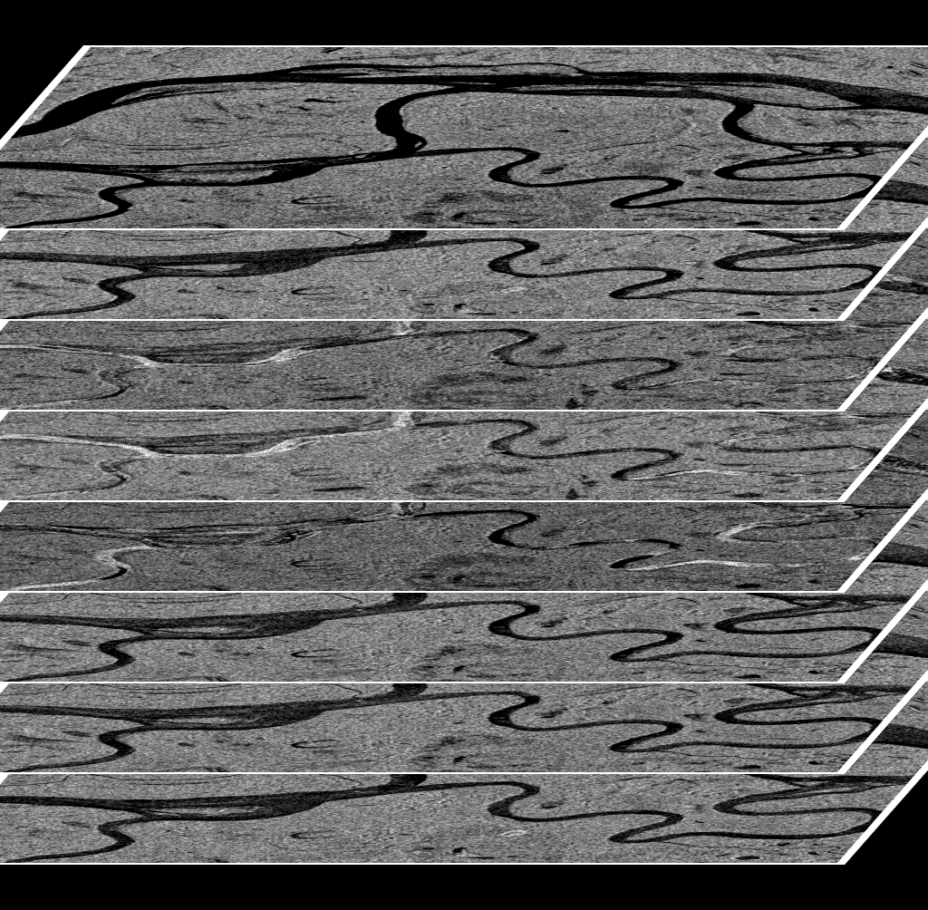
The Yukon river flats near Beaver, Alaska. ASF DAAC 2019, contains modified Copernicus Sentinel data 2017-2018, processed by ESA.
Click image for animation.
The Bering Glacier in Alaska. Drastic darkening and lightening occur throughout the seasons based upon the wetness of the glacier surface. ASF DAAC 2019, contains modified Copernicus Sentinel data 2018-2019, processed by ESA.
ASF MapReady
Terrain-correct, geocode, and apply polarimetric decompositions to multi-pol synthetic aperture radar (SAR) data
The MapReady Remote Sensing Tool Kit allows users to process SAR data from a variety of missions, including datasets served by ASF and other providers, and some optical data. MapReady is particularly useful for working with SAR datasets delivered in CEOS format.
Note that MapReady is not suitable for processing Sentinel-1 products. The platform that MapReady supports is limited to older missions in ASF’s catalog, including ALOS Palsar. Use the Sentinel-1 Toolbox packaged in the Sentinel Application Platform (SNAP) for processing Sentinel-1 data.
- Terrain-correct, radiometrically correct, geocode
- Apply polarimetric decompositions to multi-pol SAR data
- Export to a variety of common imagery formats including GeoTIFF, JPEG, PNG
- Perform basic geocoding (with no terrain correction)
- Geocode to a constant elevation
Other software included in the package are an image viewer, metadata viewer, a projection coordinate converter, and a variety of command line tools.
MapReady for Linux latest version (beta)
GitHub download site
MapReady for Windows 3.2.1 (beta)
Download
How you install the tool depends on which operating system you are using. Windows packages come with an installer, Linux packages come as an RPM, and Source packages contain source code with an autoconf-style configure script.
Windows Installation
The Windows package contains just a single file, the installer. To install, download the desired Windows version using the links above, open the downloaded file (double-clicking on it will open it), and run the installer program contained within. If running Windows 7, you will need to install the package as administrator: right-click the installer and select the Run as Administrator option.
After installation, the MapReady software is contained in a start-menu group called ASF Tools, which contains the following:
- ASF MapReady: the main software program (formerly known as “Convert)
- ASF MapReady Manual: an extensive PDF document that describes all of the installed programs and contains examples of their use
- ASF View: a viewer application capable of displaying a variety of SAR data formats, including CEOS, GeoTIFF, ASF Internal Format files
- CEOS Metadata Viewer reads the CEOS leader file which contains the metadata associated with the binary data and has both binary and ASCII components
- Projection Coordinate Converter: a utility for converting coordinate values from one map projection to another
By default, the installer also creates desktop icons for MapReady and ASF View.
Linux Installation
To install the RPM, you must have root access. If you do not, you will need your system administrator to install the package for you. If this is not feasible, the Source package can instead be downloaded, compiled, and installed in your own home directory, which does not require root privileges.
To install the package:
1. Extract the RPM from the archive:
gunzip mapready-X.X.X-linux.tar.gztar xvf mapready-X.X.X-linux.tar
2. As root, install the RPM:
rpm -i asf_mapready-X.X.X-1.i386.rpm
(Replace the Xs with whatever version you downloaded, for example: “rpm -i asf_mapready-2.0.5-1.i386.rpm”)
3. Locate the directory containing the installed package. After the package is installed, you can find the location of the installed components by using this RPM command, which does not require root access:
rpm -ql asf_mapready | grep asf_import
You should see something like the following:
/usr/local/bin/asf_import
which tells you that the package has been installed in /usr/local, which is the default.
4. Add the directory containing the installed package to your path in order to run the tools. The method of adding a path depends on which UNIX shell you are using.
For example, suppose the software was installed in /opt/asf_tools. For sh, ksh, bash, or similar shells, add these lines to your ~/.profile or ~/.bashrc file:
PATH=/opt/asf_tools/bin:$PATHexport PATH
For csh or tcsh, add this line to your ~/.cshrc file:
setenv PATH /opt/asf_tools/bin:$PATH
If you’ve gone with the default installation location of /usr/local, you may already have /usr/local/bin in your path, in which case you don’t need to do anything.
Source Installation
Required packages to build ASF tools:
- GCC
- GCC-C++
- pkgconfig
- automake
- autoconf
- gtk2-devel
- libglade2-devel
- Glade2
- Bison
- Flex
After you’ve downloaded the archive, you need to extract the package and compile the tools before they can be installed. To do this, make sure you’re in the directory containing the downloaded archive, then follow the following steps:
1. Extract the directory tree from the archive:
gunzip mapready-X.X.X-src.tar.gztar xvf mapready-X.X.X-src.tar
2. Build the tools. Please note that you will need permissions to put files into [[installation location]]! The default is /usr/local.
cd asf_tools./configure --prefix=[[installation location]]make
3. Install the tools
make install
4. Include the tools in your path. You do this one of two ways depending on the UNIX shell you are using.
For sh, ksh, bash, and similar shells, add the following lines to either the ~/.profile or ~/.bashrc file.
PATH=[[installation location]]/bin:$PATHexport PATH
For csh or tcsh, add this line to the ~/.cshrc file:
setenv PATH [[installation location]]/bin:$PATH
For example, say you would like to install the tools in a folder called “asf_tools” in your home directory (/home/jdoe/asf_tools), and you use the bash UNIX shell
./configure --prefix=/home/jdoe/asf_toolsmakemake installecho "PATH=/home/jdoe/asf_tools/bin:$PATH" >>~/.bashrcecho "export PATH" >> ~/.bashrc
MapReady 3.2.1 (beta) (released 2013 June 27)
New Functionality
- Support for Seasat HDF5 data in ASF View and MapReady.
MapReady 3.1.24 (released 2013 June 14)
New Functionality
- Now allow export of the incidence angles even when not performing radiometric terrain correction.
MapReady 3.1.22 (released 2012 December 21)
New Functionality
- Enhanced support for ingest and terrain correction of PolSARPro data, including radiometric terrain correction
- Support for geocoding to geographic coordinates
- Support use of ERS-1 and -2 precision state vectors
- Added ability to account for the geoid during terrain correction
- No longer support pixel size specification for terrain correction, software will choose appropriate size
- Enhanced support for UAVSAR, TerraSAR-X and RADARSAT-2 data (MapReady has limited support for RADARSAT-2 data)
Bug Fixes
- Fixes in geolocation of PALSAR L1.1 (SLC) data
Known Issues
- UAVSAR geolocation for .mlc files off. Use .grd files when possible.
- Windows MapReady *.meta file not being removed (or in wrong location) after processing PolSARPro files.
- Some color differences between MapReady output and the PolSARPro .bmp files may be seen. This is due to different mapping methods.
MapReady 3.1.19 (beta) (released 2012 December 4)
New Functionality
- Enhanced support for ingest and terrain correction of PolSARPro data, including radiometric terrain correction
- Support for geocoding to geographic coordinates
- Support use of ERS-1 and -2 precision state vectors
- Added ability to account for the geoid during terrain correction
- No longer support pixel size specification for terrain correction, software will choose appropriate size
- Enhanced support for UAVSAR, TerraSAR-X and RADARSAT-2 data (MapReady has limited support for RADARSAT-2 data)
Bug Fixes
- Fixes in geolocation of PALSAR L1.1 (SLC) data
Known Issues
- UAVSAR geolocation for .mlc files off. Use .grd files when possible.
- Some PolSARPro parameter results will be all-black.
- Occasional failures in the TerraSAR-X data ingest.
MapReady 3.0.6 (released 2012 May 4)
New Functionality
- Support for UAVSAR data
- New radiometric terrain correction method (Ulander)
Bug Fixes
- Fixed a number of problems with geolocation of PALSAR L1.1 (SLC)
Known Issues
- KML overlay generation fails for images that cross the dateline.
- Workaround: Turn off thumbnail and overlay generation for these files. OR Ignore the error, the desired output file has been generated even though the processing resulted in an error and didn’t move to “Completed”.
- Unable to “Add Output File Prefix or Suffix” for PolSARPro Covariance matrix files.
- Workaround: Do not use the feature for these files.
- MapReady does not always warn me if I am about to overwrite previous files.
- Additional Info: This can occur when the input has multiple bands that each need to be calibrated, so that you get multiple output files with band suffixes appended.
- Workaround: When re-processing files, make sure you’ve saved any files from previous runs.
- MapReady does not always delete intermediate files.
- Additional Info: During processing, MapReady creates a temporary directory in the directory where the final output will be put, containing intermediate files. Sometimes these directories are not cleaned up properly after processing.
- Workaround: They can be ignored, however if disk space becomes an issue they can be deleted manually.
- Thumbnails are not generated for all product types.
- Additional Info: For AIRSAR, ALOS Mosaic files, and some UAVSAR files, the input and output thumbnail are not generated in the GUI.
- Workaround: Use “View Input” or “View Output” to look at the files.
- ‘Error: This data cannot be calibrated, missing calibration block.’ encountered while attempting to generate a Sigma Radiometry image of AIRSAR data.
- Additional Info: AIRSAR data is already calibrated, and MapReady cannot re-calibrate it. The GUI should prevent attempting to do so but currently does not.
- Workaround: Do not attempt to calibrate AIRSAR data, it is not necessary.
- Unable to open a file in the Completed Files section in Google Earth.
- Additional Info: In the MapReady console window, you will see the name of the KML file MapReady is trying to open. Sometimes, this is not the name of the actual KML file that was generated.
- Workaround: Go to the output directory, and double-click the actual KML file to open it in Google Earth.
- Faulty error message for PolSARPro data with colormap and export to floating point GeoTIFF.
- Workaround: In Export tab, check Output data in byte format (instead of floating point).
- Pixel values of radiometrically terrain-corrected PolSARPro T3 matrix differ greatly from those of geometrically terrain-corrected T3 matrix.
- Workaround: Not supported for PolSARPro files.
- Calibration of all PolSARPro files processed exhibits unexpected values.
- Workaround: Calibration is not necessary for PolSARPro files.
MapReady 2.3.17 (released 2010 December 10)
New Functionality
- Added the Combine command for mosaicking images which have been geocoded with the same map projection parameters. Only available at command line.
- Enhanced map projection support by adding the native datums ITRF97, ED50, and SAD69 to the predefined map projection parameter files.
- Enhanced export to GeoTIFF format to incorporate map projection enhancements.
- Changed the default number of looks value from 8 to 7 for ALOS PALSAR quad-pol data.
- Added map distortion parameters to Information Window in asf_view.
- Extended the functionality of asf_kml_overlay.
- Now supports native PolSARPro format (geocoded data only).
- Added -reduction_factor option for resizing the overlay.
- Added -transparency option to define the opacity of the overlay.
- Added -colormap, -rgb, and -polsarpro options to generate color-coded PolSARPro data.
- Added thumbnail views for RADARSAT-2 data. (MapReady has limited support for RADARSAT-2 data.)
- Support for ingesting and viewing ROI_PAC files.
- Additional support for processing GAMMA interferometric files.
- Added InSAR block to metadata structure to display image and baseline information.
Bug Fixes
- Fixed metadata so that correct beam mode is displayed for ALOS PALSAR data.
MapReady 2.3.6 (released 2010 February 1)
New Functionality
- Generation of KML overlays.
- Support for the Equirectangular and Mercator projections.
- Support in the MapReady GUI for the ALOS KC mosaics.
- Ability to terrain-correct in flat areas, via the “Skip coregistration when it fails” option.
- Support for some TerraSAR-X and RADARSAT-2 data. (MapReady has limited support for RADARSAT-2 data.)
- PALSAR calibration updated according to latest JAXA specifications.
- Support for ingest of more types of PolSARPro data in the MapReady GUI
- Support for export to PolSARPro format.
Bug Fixes
- Geocoding of dB values was slightly off
MapReady 2.2.5 (released 2009 May 23)
New Functionality
- New ‘external’ tab in the MapReady GUI, allows running of a command-line tool after import, prior to terrain correction or polarimetric processing.
- Support for ingest of PolSARPro data in the MapReady GUI
- Improved radiometric terrain correction (new correction formula)
- Experimental support for TerraSAR-X and GAMMA data
- New Tool: diffimage (reports statistical differences in b/w images)
- New Tool: diffmeta (report differences in metadata files)
- New Tool: adjust_bands (allows combining/reordering/removing bands in multi-band files)
MapReady 2.1.11 (released 2009 March 30)
New Functionality
- New Polarimetric Decompositions:
- The Cloude-Pottier decomposition, with 8 or 16 classifications, as well as the raw entropy/anisotropy/alpha values.
- Freeman-Durden
- Faraday Rotation correction
- In ASF View, the ability to overlay a shapefile, or a generic CSV file, on top of the image.
- Support for ingesting GeoTIFFs which use angular pixel sizes.
- Support for viewing certain useful intermediate files generated during processing.
- MapReady now thumbnails GeoTIFFs loaded into the input file list.
- GUI support for AIRSAR data (interferometric)
- Added support for ERSDAC ALOS mosaics
- New Tool: brs2jpg, converts ALOS .BRS files to jpeg.
Bug Fixes
- Eliminated streaking at the edge of an image with some RADARSAT-1 SLC data
- Changing the output directory during processing no longer breaks use of the “View Output” or “View Metadata” options.
MapReady 2.0.13 (released 2008 August 27)
New Functionality (GUI and command-line tools)
- Support for single-look complex (SLC) data, including PALSAR Level 1.1.
- Allow processing quad-pol (PALSAR Level 1.1, 1.5) data into the Sinclair polarimetric decomposition
- Allow processing quad-pol SLC (PALSAR Level 1.1) data into the Pauli polarimetric decomposition
- Implemented correction for the ERS-2 gain loss.
- Use the new ALOS 25-parameter transform block, available in data produced by the ALOS processor 9.0+. Significantly improves geolocation of ALOS data.
- Support in asf_terrcorr for skipping the coregistration and using user-supplied offsets.
- Support for use of DEMs in the lat/lon pseudoprojection during terrain correction.
- New Tool: asf_proj2proj is a command-line interface to the ASF Projection Coordinate Converter.
- In ASF View, allow the user to move the crosshair to a specified lat/lon, line/sample, or projected x/y coordinate.
- Support for AIRSAR data. [command-line only]
- Support for Gamma data. [command-line only]
Bugs Fixed
- When using “Save Clipped DEM” with terrain correction, the saved DEM was not always clipped properly.
- MapReady would crash on Windows Vista.
- MapReady’s “Help” option would not work on Windows Vista.
- ASF View would not always find the CEOS Metadata file when that button was clicked.
- ASF View’s “Save Subset” option would produce invalid ASF Internal files when generated from CEOS images.
- ASF View’s “Save Subset” option would have incorrect geolocations when used on projected data.
- Projection converted would not detect the zone when converting back to UTM from lat/lon.
Features Enhanced
- On Windows, changed to use the GTK+ browse-for-folder widget when using the “Browse” button on the “Destination Folder” dialog, instead of the Windows one. Allows creating directories within the widget, and can be set to start up in the current directory.
- Allow terrain correction of calibrated and polarimetric data by adding an amplitude band that is used only for coregistration.
- Include processing settings and timing information in the MapReady log file.
- Geocode would produce grainy results when significantly downsampling.
- Improved ASF View’s depiction of RGB images by using separate contrast expansion on all three bands, instead of a single mapping for all three.
- Pixel averaging in ASF View when zoomed out. (Results in a less grainy image.)
MapReady 1.0.4 (released 2008 May 23)
New Functionality
- Added support for user-defined UTM projections used by GRASS.
- Metadata Viewer: Added support for the JAXA Facility Data Record.
Bugs Fixed
- Fix crash when selecting PALSAR IMG- file under some circumstances.
- Fix problem viewing help under Vista.
- Fix core dump importing USGS DEM under Solaris.
- Some UTM DEMs using NAD27 were being incorrectly interpreted as WGS84.
- Error out when trying to import SLC data, as this is not supported for 1.0.
- Error out when trying to import Level 0 data, as this is not supported for 1.0.
- Error out gracefully (instead of crashing) when trying to terrain-correct with DEMs in the Lat/Lon pseudoprojection.
- Use a different transformation block when geocoding PALSAR data. Should improve PALSAR geolocations, particularly at higher latitudes.
- Fix some incorrectly populated metadata fields for CDPF SSG data.
- Fix some incorrectly populated metadata fields for RSI SGF data.
- GeoTIFF import was not populating False Easting/Northing for some files using Lambert Conformal Conic.
- ASF View: Can now view non-map-projected TIFFs
- ASF View: Fixed incorrect distance reported when trying to measure across a UTM zone boundary.
MapReady 1.0.3 (released 2008 February 12)
New Functionality (GUI and command-line tools)
- Added GeoTIFF DEM ingest support to asf_import
- New installer scripts for all tools
Bugs Fixed
- Some documentation topics were clarified (.meta files, ASF Internal format description)
- Location block in metadata not populated when importing certain RSI data
- Metadata viewer failed to display the data set summary record for certain CDPF data
- Configure script improved so that if GTK libraries are not available, it is made very clear that the applications with graphical user interfaces will not be built
- Some polar stereographic map projected data sets would not reproject
- Some polar stereographic SSM/I map projected data sets failed to import or imported with scaling errors
- Improved tool tips in MapReady GUI
- Better file clean up (temporary thumbnail files)
- asf_import failed to process long STF swath
- Resolved build errors for building on Sun Solaris v8 and v9 systems
- asf_geocode failed for missing projection parameters (parameters that could be surmised from existing information)
- Some ALOS L1.5 data failed to reproject
MapReady 1.0.2 (released 2008 January 2)
New Functionality (GUI and command-line tools)
- Convert GUI name changed to MapReady and redesigned and reorganized the user interface for more intuitive use, advanced tool tips, improved help. Command line version, asf_convert, renamed to asf_mapready.
- New Tool: Added new SAR and Optical image viewer (asf_view). Replaces, modernizes, and enhances capabilities previously found in the now-unsupported sarview tool, allows viewing geographic regions covered by the dataset in Google Earth, and applies pseudo-color according to look-up tables available from a drop-down list.
- New Tool: Added shift_geolocation (command line) to the toolset. Allows manual shifting of geolocation if a known offset exists. Similar to refine_geolocation but no DEM is required.
- New Tool: Added Projection Coordinate Converter (GUI) to the toolset. This tool converts projection coordinates in one map projection into projection coordinates in another map projection. The GUI allows you to specify map projection parameters, manually enter coordinates, or select a file that contains coordinate triplets (x, y, height) — one triplet per line. Results can be saved to a file as well.
- New Tool: Added ‘trim’, a simple command-line utility that facilitates subsetting an ASF Internal Format file given starting line, number of lines, starting sample, and number of samples.
- New Tool: Added ‘fill_holes’, a tool that replaces values in an image below a given cut-off with values interpolated from the shape and height of the surrounding terrain. The fill_holes tool is handy for manually patching ‘holes’ (regions with no-data values, typically very small negative values) in DEMs prior to using the DEM for terrain correction. The result is that hole-related artifacts in terrain-corrected images are minimized (available as a command-line flag to asf_mapready and as a checkbox in MapReady as well.)
- New Tool: The ‘to_sr’ tool has been added to the tool suite. The to_sr tool converts a ground range (or map-projected ASF Internal format image with state vectors available in the metadata file) into a slant-range image. Replaces deprecated gr2sr tool.
- New Tool: The ‘deskew’ tool has been added to the tool suite. The deskew tool removes satellite platform squint-induced skew from ground range images.
- Enhanced TIFF/GeoTIFF ingest to support a much broader spectrum of GeoTIFF types (scanline, tiled, striped, color; geocentric lat/long in decimal degrees)
- Added support for several new CEOS data formats (BEIJING ESA raw, CDPF)
- Terrain correction of ScanSAR and ALOS PALSAR
- Sinclair decomposition upon export for real-valued radar images
- Added ‘Display in Google Earth’ buttons to the GUI for viewing of the data extents in the Google Earth ™ program.
- Added ability to patch ‘holes’ (interpolate over missing data) in DEMs. Also, see new tool ‘fill_holes’.
- Ability to export PNG graphics file format
Bugs Fixed
- Resolved some minor memory leaks
- shift_geolocation now works properly on map-projected images
- Fixed several (minor) metadata inconsistencies
- Resolved 700 m to 1.5 km geolocation offset which occurred in some ALOS AVNIR2 images
- Resolved file seek error which occurred when importing into a sigma nought power image
- Resolved band_count error when importing GeoTIFFs with empty color channels
- USGS Seamless Server DEMs in GeoTIFF format are now in tiled TIFF format. Importing this format is now supported.
- Resolved issues with geocoding images that cross the zone 1 to 60 boundary in UTM map-projections.
- Resolved minor inaccuracies in ScanSAR alpha-rotation projections.
Features Enhanced
- Improved Windows registry settings to allow parallel installations of multiple versions of the tool set (including uninstallation)
- Import of polar stereographic SSM/I CEOS data now defaults to utilizing the Hughes reference spheroid
- Enhanced import/export of image bands (channels, polarizations, etc)
- Added support in the command line version of asf_convert for exporting individual bands from multi-band files
- Improved JPEG output (reduced JPEG artifacts)
- Metadata now includes location block (corners, center, lat/long)
- Made input file name specification more flexible and removed some dependencies on the name of the file (less error prone)
- Added support for a broader variety of input file naming conventions
- Added support for bicubic resampling during geocoding of byte images
Note: Although some answers on this page are outdated, users report they are useful enough to retain while ASF works on updates. Users may contact ASF with further questions.
Documentation and Terminology
- Where do I find the documentation for MapReady?
- In Windows the PDF version of the comprehensive manual is located in the ‘Start’ menu at ‘Programs -> ASF tools -> MapReady’. In Linux the documentation is located in /usr/local/share/asf_tools/doc (assuming that the tools were installed by the system administrator).
- Where can I find the details about the satellite metadata?
The ALOS production specifications for the different sensors are provided by JAXA:
For other data formats please see:
- What do the different levels in optical ALOS data mean?
There are four levels of ALOS AVNIR/PRISM data:
- level 0: raw data generated by every downlink segment and every band
- level 1A: raw data extracted from level 0, expanded and generated lines
- level 1B1: radiometrically corrected image
- level 1B2R: geometrically corrected image, georeferenced (corner coordinates known in map projection)
- level 1B2G: geometrically corrected image, geocoded to map projection
- Can you tell me the difference between pixel spacing and pixel size of SAR image?
- I would use the terms “pixel spacing” and “pixel size” interchangeably. The terms that usually mixed up are is “pixel size” and “resolution.” Resolution refers to the size of the resolution cell on the ground, i.e. the area where the information in your pixel came from. The pixel size depends on what the processor does with that. Usually the pixel size is smaller, i.e. the processor oversamples the information that it has.
- In a file it is said that for PALSAR SLC polarimetric image, its pixel spacing is 9.36 m in range direction, and it is 1.77 m in azimuth direction. Is it right?
- SLC stands for single look complex, i.e. the image has not been multilooked. Therefore, you are dealing with pixels that are not square (yet). Regular detected products come with a square pixel size. If you look at the amplitude image from your SLC image, you will see that everything is stretched in azimuth direction. Depending on the type of polarimetric data (single-pol, dual-pol or quad-pol) you have a ratio of 1:8 or 1:4 to get to square pixel by multilooking.
- What is Faraday rotation?
- Faraday rotation is a rotation of the polarization vector of radio waves that propagated through the ionosphere. L-band SAR data such as ALOS PALSAR data are most affected by this.
Software and Functionality
- What data formats are currently supported?
- This table summarizes the data formats:
Format Import Export Comments CEOS x Sky Telemetry Format x GeoTIFF x AIRSAR polarimetric x AIRSAR InSAR x TerraSAR-X x Gamma x PolSARpro x ALOS mosaic x Vexcel Plain x BIL x has not been tested lately GridFloat x has not been tested lately JAXA L0 (optical) x ENVI x x ingest in asf_view TIFF x JPEG x PNG x PGM x ALOS browse image x direct conversion to JPEG
- What CEOS flavors are supported?
- This table summarizes the supported CEOS flavors:
Facility Products Comments ASF PP ERS-1, ERS-2, RADARSAT-1, JERS-1 JERS-1 L0 to be verified ASF SSP all products EOC PALSAR (level 1.1, level 1.5) single-, dual- and quad-pol EOC PRISM (1A, 1B1, 1B2R, 1B2G) 1A and 1B1 only import EOC AVNIR (1A, 1B1, 1B2R, 1B2G) 1A and 1B1 only import D-PAF RAW, SLC I-PAF RAW, SLC ESA RAW, SLC CDPF SLC, SGF, SGX, SSG, ScanSAR RSI RAW, SGF, SGX, ScanSAR CSTARS RAW, SLC, SGF, SGX, PRI, SSG, GEC, ScanSAR work in progress Beijing RAW Tromso SNA, SNB Westfreugh SNB Dera PRI
- What calibration schemes are supported?
- This table summarizes the supported calibration schemes:
Type Calibration projection Comments ASF sigma linear equation (includes noise floor) ESA gamma constant ALOS sigma constant CDPF gamma range dependent look up table
- What Linux operating systems can I use to build MapReady from source?
- You can probably compile the tools on any Linux system. We develop the tools on CentOS and Ubuntu machines (32-bit and 64-bit).
- Does MapReady work on a Mac?
- We managed to compile the command line tools on a Mac, but this operating system is currently not supported.
- How do I launch a tool under Windows?
- The graphical user interface in MapReady (ASF MapReady, ASF view, CEOS Metadata Viewer, Projection Coordinate Converter) are by default in the Start menu ‘Programs -> ASF tools > MapReady’. The command line tools can be launched from the MS-DOS prompt. To open the MS-DOS prompt, you click ‘Run’ and type ‘cmd’.
- I am trying to process my data with MapReady and get a “permission denied” error. Why is that?
- The most likely cause for this is that you are trying to process data that is on a DVD. By default, MapReady selects the output directory where the input data is. Since our data DVDs are read only, you don’t have permission to write to them. As a minimum, you want to change the output directory that is located on a regular hard disk. Alternatively, you can copy the data from DVD to your computer before you do the processing.
- Is there a way to help the developers help troubleshooting a problem with MapReady?
- Most definitely. A screen capture of the exact error message is a good starting point. The log file of the problem run gives us even more information. The best way to even troubleshoot a problem yourself, besides looking at the log file, is to use the “Keep intermediates” option in the general settings of MapReady. The log file indicates the commands used in the processing flow with some indication what files were used. The more information we have, the easier it is to reproduce the problem on our end, in order to figure out what is wrong.
- Where do I find intermediate results?
- For processing each data set MapReady generates a temporary directory such as “ALPSRP106002960-P1.5_UD-08-Apr-2009_15-15-38”. The directory name contains the name of the file and a time stamp when the data set was processed. This way you are not accidentally overwriting any previously processed results. Unless the user specifies that this directory is kept with the “Keep intermediates” option in the general settings, the directory is deleted.
- What does “temporarily keep intermediate files” mean?
- Intermediate files are kept until program exit, or the file is removed from the “Completed Files” section, to allow viewing the intermediates after the processing has completed.
Data Support and Metadata
- What kind of SAR data does MapReady ingest?
- Data in CEOS and in Sky Telemetry Format (STF).
- What type of CEOS data is supported?
- MapReady supports three types of CEOS data. The CEOS level zero data is raw signal data that needs to run through a SAR processor before it can be visualized. CEOS single look complex (SLC) data is primarily used for SAR interferometry, as it contains both amplitude and phase information. CEOS level one data is the most commonly used for all other applications.
- Does MapReady support CEOS data formats other than ASF’s?
- We have incorporated generic support for a number of other CEOS flavors. If you have a data set that does not ingest, please provide us with the data set, so that we enhance the ingest capabilities in future releases. These efforts progress as time permits.
- Can MapReady handle ScanSAR level zero data?
- The processing of ScanSAR raw data is not supported. The ScanSAR data consists of several bands (the numbers varies between three and five depending on the satellite) that are processed separately and then “stitched together.” That is beyond the capabilities of our regular SAR processor.
- Does MapReady ingest ALOS PALSAR Level 1.0?
- No, it doesn’t. MapReady support starts with level 1.1 data.
- Which types of optical ALOS data is supported by MapReady?
- Only level 1B2 data are supported, regardless whether they are georeferenced or geocoded.
- Does MapReady support RADARSAT-2 data?
- No, it does not.
- Does MapReady support SIR-C data?
- Not at this point.
- I want to have a look at the CEOS metadata. How do I do that?
- There are two ways of going about it. There is a graphical user interface that is located in the Windows ‘Start’ menu at ‘Programs -> ASF tools -> CEOS metadata viewer’. From the command line you can start it by typing mdv. Alternatively, the command line tool metadata allows you to extract the individual CEOS records out of the leader file. They can also be saved as plain text files.
- I have lot of SAR data to analyze. Is there a way to extract from such as corner coordinates for each scene?
- You want to use is the convert2vector tool. With a larger number of files you want to use the ‘-list’ option that reads the input from a text file that contain the list of files to be converted. The input format option would be ‘leader’ and the output format option would be ‘csv’. That would dump the coordinates (and other relevant metadata) to a comma delimited ASCII text file. This is assuming that you want to parse the information to some other application. For visualization purposes you choose the output as KML or shape file.
Data Analysis
- I want to do some analysis with my SAR data that requires parameters such as sigma0 and incidence angle. What type of data should I use?
- This type of analysis requires detected (L1) data. Since the data is not geocoded yet, it still contains all the information about the viewing geometry.
- I need to create a subset of my data. Which tool should I use?
- There are two tools that generate subsets: trim and asf_view. If you just want to work with the pixel values of an image, trim is the faster solution. If you want additional information such as geometric parameters for the subset, you want to use asf_view.
How do I extract incidence angle information out of my data?
After loading the image in asf_view, you can extract a subset for which you can save a number of values. In order to define the subset in the viewer, you place a crosshair for one of the corner points of your area of interest (left-click). Then you keep adding points to the polygons (ctrl-left-click).
The list of values that you can save for an image subset include
- pixel values
- incidence angle
- look angle
- slant range
- time
- Doppler
- scaled pixel values
- In what format can I save subsets generated with asf_view?
- Subsets can be saved in the ASF internal format or a command delimited text file (CSV).
- Can I apply speckle filtering in MapReady?
- We have not implemented any speckle filters in MapReady, neither for regular nor for polarimeteric processing.
Radiometry and Calibration
- What is getting calibrated? The data or the processor?
- A SAR processor is calibrated when the coefficients required for accurate radiometry have been determined, but an image is calibrated only when those coefficients have been applied.
- I have three options for the radiometry to choose from? Which one do I need?
- It depends on what you want to do with the data.
- Beta nought is essentially a ratio between the power that was sent from the antenna and the power that returned to the antenna. Beta nought is in the realm of slant range. This is typically used by engineers that care about the electronics of it all.
- Sigma nought is the power returned to the antenna from the ground plane and is thus in the realm of ground range. Scientists tend to use this measure.
- Gamma nought is typically used when calibrating the antenna. Since each range cell is equally distant from the satellite, near range and far range are equally as bright which is helpful in determining the antenna pattern.
- I have some calibrated SAR data but the value range (0 to 5) does not look right. Are these values in dB?
- The value range suggests that your values are in power scale. In order to get them into the dB scale, you would need to convert them:
dB = 10 * log10 (power scale)
A value range in power scale between 0 and 5 would be equivalent to a value range between -50 dB and 0 dB.
- I want to know the average backscatter value of an area in dB. How do I do that?
- You apply the calibration parameters by selecting the radiometry to be ‘Sigma’, ‘Beta’, or ‘Gamma’ and ingest the data. This will result in an image in power scale values. Do not scale the output to decibels. Average the values in the area of interest and convert the average value to dB, using this formula:
dB = 10 * log10 (power scale)
- I want to analyze my calibrated backscatter values in another software package. What export options should I choose?
- In order to ingest your data properly in any of the image processing and GIS software packages out there, you want to export your geocoded data into GeoTIFF format. That is probably the best supported format that contains all the relevant map projection information. In order to keep the full dynamic range and the original values you want to export the data as floating point data. So do not scale your data to byte values.
- I heard ERS-2 data sets have a gain loss problem. Can I correct my ERS-2 data for that?
- The ERS2 satellite has a known gain loss problem. All pixels in the image are scaled by a correction factor that is date-dependent. This is only applied to calibrated data.
Polarimetry
- What kind of data do I need for polarimetric processing in MapReady?
- You need fully polarimetric single look complex (SLC) data. For ALOS PALSAR data that means level 1.1. Polarimetric AIRSAR data is also supported.
- I have some dual-pol data. Can I use those for polarimetric processing?
- Dual-pol data is not supported for polarimetric processing within MapReady. However, this type of processing can be done in PolSARpro and ingested into MapReady after that.
- Is there any polarimetric decomposition that works with ALOS Palsar level 1.5 data?
- The only polarimetric decomposition that also works with detected imagery is Sinclair.
- What do the colors in the Pauli decomposition mean?
- Each color represents a different scattering mechanism (Red: even, Green: volume, Blue: odd).
- What parameters are calculated for the Cloude-Pottier decomposition and what do they mean?
- These parameters are calculated from the coherence matrix, which is calculated for each pixel. These parameters are “entropy,” “anisotropy,” and “alpha.” Entropy is an indication of the degree of randomness in the scattering process. Low entropy means there is a single dominant scattering mechanism in that pixel; high entropy means multiple scattering mechanisms are present in the pixel. Anisotropy represents the relative importance of the non-dominant scatterers. When entropy is low, the anisotropy parameter means very little, but for high entropy it is a useful indication of the strength of the secondary scatters. Alpha can be used to identify what type of scatterer is the dominant one. When alpha is close to 0, single-bounce scattering (e.g., a rough surface) is dominant. For alpha near 90°, the dominant scatterer is double-bounce. Alphas in between these extremes represent a combination of both; at 45° we have equal amounts of both which usually corresponds to volume scattering.
Digital Elevation Models (DEMs) and Terrain Correction
- What kind of digital elevation models (DEMs) should I use for terrain correction?
- For the U.S., the data is available in 30 m spacing. For the rest of the world between 60 degrees northern latitude and 56 degrees southern latitude the data is available in 90 m spacing.
- My DEM downloaded from the National Map Seamless Server does not work in the terrain correction of MapReady?
- Once you’ve selected your area of interested and the download window pops up, make sure to click on the “Modify data request” link up top before you hit the download button. In the “The National Map Seamless Server Request Options Page” scroll down to your dataset and change the data format from ArcGRID to GeoTIFF. Then scroll to the bottom and click the “Save Changes & Return to Summary” button. Now you can click the download button and retrieve your GeoTIFF format DEM for terrain correction in MapReady.
- Do you know any software that will generate a DEM from an ALOS PRISM triplet?
- PCI Geomatica is able to generate DEMs from PRISM. It supports level 1B1 (preferred) and level 1B2R data.
- How many ground control points (GCPs) does PCI Geomatica take for the generation of a PRISM DEM?
- PCI recommends six GCPs per CCD.
- Is it possible to run MapReady for AIRSAR data terrain correction?
- Our current implementation of the terrain correction does not support this. However, the geocoding of AIRSAR data is supported.
- I am having trouble with one PALSAR scene in MapReady, it won’t run with the terrain correction application. With this particular image I get the error below:
- “Correlated images failed to match!
Original fftMatch offset: (dx,dy) = 1080.027343750, -492.555908203After shift, offset is: (dx, dy) = -1312.802612305, 476.835266113
- The first thing terrain correction does is create a simulated SAR image from the DEM, and then use FFTs to match this simulated image with the image you’re terrain-correcting. For this FFT matching to work, there has to be some “relief” in the scene — mountains, hills, etc. Is the scene that is failing of a flat area, and the surrounding scenes contain the hilly areas? If this is the case, you can probably just skip terrain correction for that scene — and when geocoding, specify the average height of the area.
- What kind of vertical datum is required for DEM in MapReady for terrain correction and geocoding. Geoidal height (above mean sea level) or ellipsoidal height?
- Ellipsoidal height is what MapReady is looking for.
- Are there cases when I should not terrain-correct my data?
- Terrain correction is usually not a good idea when the area of interest is very flat or does not have a lot of relief. In these cases you might consider geocoding the image to the average height.
- Is there a way to mask out an area that should not be terrain-corrected, e.g. big water bodies, or areas that are otherwise constantly moving, e.g. glaciers?
- MapReady can generate a water mask derived from a DEM, assuming the areas below a certain threshold (the default value is 1 m) is water. Other areas can be masked out based on a mask file that the user needs to supply.
- The matching of my SAR image and the simulated SAR image derived from the DEM fails, but I still see some offsets in the results. What can I do?
- You can manually measure what the offset is and apply those values in the “Skip co-registration” option.
- Why is the matching of the real image and the simulated image derived from the DEM done in slant range?
- The matching in original SAR geometry is the most straightforward way of estimating the offset.
Geocoding and Export
- What map projections are supported by MapReady?
- MapReady supports the following map projections for geocoding:
- Universal Transverse Mercator (UTM)
- Albers Conical Equal Area
- Polar Stereographic
- Lambert Conformal Conic
- Lambert Azimuthal Equal Area
- I am not sure which map projection to use. What is the best projection for my project?
- Cylindrical projections work best in equatorial areas. The Universal Transverse Mercator (UTM) projection is the most commonly used one from this family of map projections. The distortions within the UTM projection are manageable as long as the projected area is not very large. Conic projections, commonly defined with two standard parallels, are often used in the mid-latitude regions. In this case, the Albers Conic Equal Area projection preserves area, while the Lambert Conformal Conic projection preserves angles. Azimuthal projections are mostly used in the polar regions. The Polar Stereographic projection and Lambert Azimuth Equal Area projection are well known representatives of this type of projection.
- I see big geolocation errors when I am geocoding JERS-1 data. What is wrong here?
- The JERS-1 satellite at times had issues with clock errors. These time errors lead sometimes to big offset in azimuth direction (flight direction). In order to remove this shift, you need to run the data through terrain correction. In the process the shift is determined by matching the real image with a simulated amplitude image derived from the reference DEM. If the area is too flat for regular terrain correction, you may need to measure the offset manually, and then use the ‘Shift Geolocation’ option in the External tab.
- Can I re-project data with MapReady?
- Yes, you can. By selecting geocode with a different map projection for already geocoded data, MapReady will re-project the data set.
- Is there a difference in exporting an optical RGB image with the “True Color” or “False Color” instead of assigning the individual band in the “User Defined” option?
- There actually is. The “True Color” and “False Color” option apply a 2-sigma contrast expansion to each individual channel before combining them to a color image. Any user-defined color combination of channels leave the original pixel values in place.
- How can I change the size of my image during the processing?
- There are two ways of doing that. There is an external tool “Resample” that allows you to resize the image right after ingesting it, choosing a scale or dimension. Alternatively, you can geocode the image to a particular pixel size.
- Can I make sure that I keep my original pixel values during the geocoding?
- By default the geocoding will use a bilinear interpolation which changes the resulting pixel value as it takes a weighted average of four input pixels into account. In order to preserve the pixel values the “Resample” method needs to be changed to “Nearest neighbor.” In case of the geocoding of polarimetric decompositions and classifications this is enforced automatically.
- I would like to mosaic some geocoded images. How do I go about that?
- This functionality is currently only available on the command line. However, there are two ways of doing it. The mosaic tool is geocoding the data and mosaicking at the same time. This would require to define all map projection parameters on the command line. The combine tool is probably more convenient for this purpose, as is does not require any map projection information. It is assumed that all input data is already in the same map projection. That, however, can easily be achieved by using MapReady for all the processing steps from ingesting the data to geocoding them. Both tools expect to see ASF internal format data. The results still would need to be exported to GeoTIFF format to be really useful.
Interferometry
- Where can I find RADARSAT-1 interferometric baseline information?
- This information has been integrated into the URSA search and order interface. After searching data for the area of interest a link to the available baseline information is located in the upper right corner.
- Does the RADARSAT-1 baseline information cover all RADARSAT-1 data?
- The baseline information is only calculated for the data in the ASF data archive.
- Can I do interferometric processing with MapReady?
- MapReady does not support any interferometric processing. However, it supports the ingest of files (currently interferogram and coherence images) generated with the GAMMA software.
Convert to Vector
Transform point or scene information to formats compatible with Google Earth, GIS, and more
Current Version: V 2.2.4
Convert to Vector is a small program made to transform point or scene information to various other formats that are compatible with external applications such as Google Earth, GIS software such as ArcGIS, text editors, and spreadsheets.Convert to Vector 2.2.4 (released 2009 April 29)
New Features:
- Ability to convert STF files, TerraSAR-X files.
Convert to Vector 2.1.1 (released 2009 January 9)
New Features:
- Capability to convert general KML files, not just those created by Convert to Vector.
- Support for converting URSA files.
- Capability to customize which metadata fields are placed in the output file by use of a configuration file.
Initial public release: Convert To Vector 2.0.4 (2008 July 30)
ASF releases a light duty software kit, Covert to Vector. This tool transforms point or scene information to various other formats that are compatible with external applications such as Google Earth(tm), GIS software such as ArcGIS(tm), text editors, and spreadsheets. One of the primary purposes of this software is to enable users to quickly and easily view the extents of a SAR dataset or a metadata file. This is done simply by dropping the file in question into the Convert to Vector tool which can automatically detect the data type, create a new file based on the available data, and open that file in Google Earth to display the image boundaries. Of course, other transformations are possible; all the tool needs is latitude and longitude information.
ASF Software License Agreement
Copyright © 2020, University of Alaska Fairbanks, Alaska Satellite Facility. All rights reserved.
Redistribution and use in source and binary forms, with or without modification, are permitted provided that the following conditions are met:
- Redistributions of source code must retain the above copyright notice, this list of conditions and the following disclaimer.
- Redistributions in binary form must reproduce the above copyright notice, this list of conditions and the following disclaimer in the documentation and/or other materials provided with the distribution.
- Neither the name of the University of Alaska Fairbanks, nor its subunits, nor the names of its contributors may be used to endorse or promote products derived from this software without specific prior written permission.
- Redistribution and use of source and binary forms are for noncommercial purposes only.
THIS SOFTWARE IS PROVIDED BY THE COPYRIGHT HOLDERS AND CONTRIBUTORS “AS IS” AND ANY EXPRESS OR IMPLIED WARRANTIES, INCLUDING, BUT NOT LIMITED TO, THE IMPLIED WARRANTIES OF MERCHANTABILITY AND FITNESS FOR A PARTICULAR PURPOSE ARE DISCLAIMED. IN NO EVENT SHALL THE COPYRIGHT OWNER OR CONTRIBUTORS BE LIABLE FOR ANY DIRECT, INDIRECT, INCIDENTAL, SPECIAL, EXEMPLARY, OR CONSEQUENTIAL DAMAGES (INCLUDING, BUT NOT LIMITED TO, PROCUREMENT OF SUBSTITUTE GOODS OR SERVICES; LOSS OF USE, DATA, OR PROFITS; OR BUSINESS INTERRUPTION) HOWEVER CAUSED AND ON ANY THEORY OF LIABILITY, WHETHER IN CONTRACT, STRICT LIABILITY, OR TORT (INCLUDING NEGLIGENCE OR OTHERWISE) ARISING IN ANY WAY OUT OF THE USE OF THIS SOFTWARE, EVEN IF ADVISED OF THE POSSIBILITY OF SUCH DAMAGE.
Third-Party Software Tools
Free/Open-Source Tools
ERDAS ER Viewer — The ERDAS ER Viewer is an easy-to-use image viewer featuring interactive roaming and zooming with very large JPEG 2000 and ECW files.
GMT5SAR — GMTSAR is an open source (GNU General Public License) InSAR processing system designed for users familiar with Generic Mapping Tools (GMT).
InSAR ISCE — InSAR Scientific Computing Environment is a flexible and extensible computing environment for geodetic image processing for Synthetic Aperture Radar (SAR), available to WInSAR members.
LIZARDTECH GeoViewer — Display MrSID imagery, raster imagery, LiDAR point clouds, and vector overlays in one standalone application.
PolSARPro — The Polarimetric SAR Data Processing and Educational Tool aims to facilitate the accessibility and exploitation of multi-polarized synthetic aperture radar (SAR) datasets.
pyroSAR — A Python Framework for Large-Scale SAR Satellite Data Processing.
SARViews — A fully automatic processing system that produces value-added products in support of monitoring natural disasters. The SARVIEWS processor is implemented in the Amazon Cloud and utilizes modern processing technology to generate geocoded and fully terrain corrected image time series, as well as interferometric SAR data over areas affected by natural disasters.
Sentinel-1 Toolbox — A collection of processing tools, data-product readers and writers, and a display-and-analysis application to support the large archive of data from ESA SAR missions including SENTINEL-1, ERS-1 and -2, and ENVISAT, as well as third-party synthetic aperture radar (SAR) data from ALOS PALSAR, TerraSAR-X, COSMO-SkyMed and RADARSAT-2.
Worldview Quick Look Tool — This tool from NASA’s EOSDIS provides the capability to interactively browse global, full-resolution satellite imagery and then download the underlying data. Most of the 100+ available products are updated within three hours of observation.
Commercial Tools
ENVI — ENVI provides advanced, user-friendly tools to read, explore, prepare, analyze and share information extracted from all types of imagery.
ERDAS IMAGINE — ERDAS IMAGINE performs advanced remote sensing analysis and spatial modeling to create new information.
GAMMA — The GAMMA SAR and Interferometry Software is a collection of programs that allows processing of SAR, interferometric SAR (InSAR) and differential interferometric SAR (DInSAR) data for airborne and spaceborne SAR systems.
Geomatica — Geomatica is a single, integrated software system for remote sensing and image processing.
