
Contains modified Copernicus Sentinel data (2015) processed by ESA
Adapted from the 2015 European Space Agency’s Advanced Training Course on Land Remote Sensing.
◆ Advanced
In this data recipe, you will learn how to create a coherence-based multi-temporal color composite of land coverage using the ESA Sentinel-1 Toolbox.
RGB — R: Coherence, G: Average Sigma0 and B: Difference Sigma0
Background
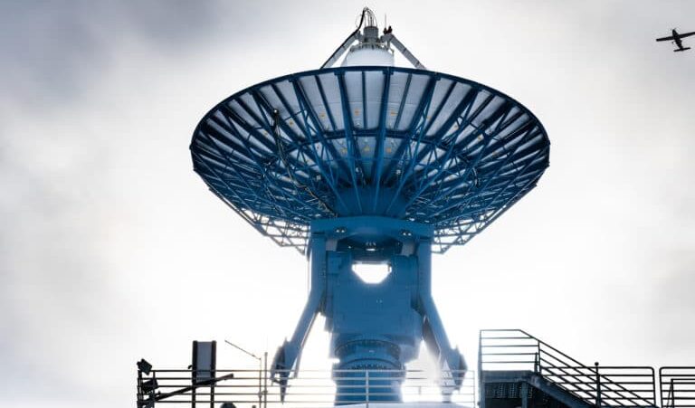
The Sentinel-1 mission comprises a constellation of two polar-orbiting satellites, Sentinel-1A and Sentinel-1B, which provide all-weather, day-and-night radar imaging for land and ocean surfaces, monitoring the marine environment, vegetation mapping, and other major applications.
With multi-temporal analyses, remote sensing gives a unique perspective of how cities evolve. The key element for mapping rural to urban land use change is the ability to discriminate between rural uses (farming, pasture, forests) and urban use (residential, commercial, recreational). Remote sensing methods can be employed to classify types of land use in a practical, economical and repetitive fashion, over large areas.
A Word on Sentinel-1 Interferometric Wide Swath (IW) Data
The Interferometric Wide (IW) swath mode is the main acquisition mode over land for Sentinel-1. It acquires data with a 250km swath at 5m x 20m spatial resolution (single look). IW mode captures three sub-swaths using the Terrain Observation with Progressive Scans SAR (TOPSAR) acquisition principle.
With the TOPSAR technique, in addition to steering the beam in range as in ScanSAR, the beam is also electronically steered from backward to forward in the azimuth direction for each burst, avoiding scalloping and resulting in homogeneous image quality throughout the swath. A schematic of the TOPSAR acquisition principle is shown to the right.
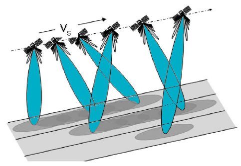
The TOPSAR mode replaces the conventional ScanSAR mode, achieving the same coverage and resolution as ScanSAR, but with nearly uniform image quality (in terms of Signal-to-Noise Ratio and Distributed Target Ambiguity Ratio).
IW Single Look Complex (SLC) products contain one image per sub-swath and one per polarization channel, for a total of three (single polarization) or six (dual polarization) images in an IW product.
Each sub-swath image consists of a series of bursts, where each burst has been processed as a separate SLC image. The individually focused complex burst images are included, in azimuth-time order, into a single sub-swath image with black-fill demarcation in between, similar to ENVISAT ASAR Wide ScanSAR SLC products.
Prerequisites
Materials List
- Windows or Mac OS X
- Multi-Temporal Sentinel-1A SLC Products
Sample Pair 1
Sample Pair 2
- Sentinel-1 Toolbox (version 5.0.0)
Note: You will be prompted for your Earthdata Login username and password, or must already be logged in to Earthdata before the download will begin.
System Requirements
The Sentinel-1 Toolbox is a very computer resource-intensive program and some steps can take a very long time to complete. Here are some hints to help speed things up and keep the program from freezing.
- Have at least 16 GB memory RAM
- Close other applications
- Do not use the computer while a product is being processed
Part 1: Processing SLC Image Pairs
Part 1 must be completed for each pair of images. You will do Part 1 twice — once for each pair.
Download Software and Data
- Download and install the Sentinel-1 Toolbox (select the correct version for your operating system)
- Create a working folder for the Sentinel-1 sample images and intermediary products created during processing
- Download the sample images from the Materials List and place them in the new working folder
Open Data in Sentinel-1 Toolbox
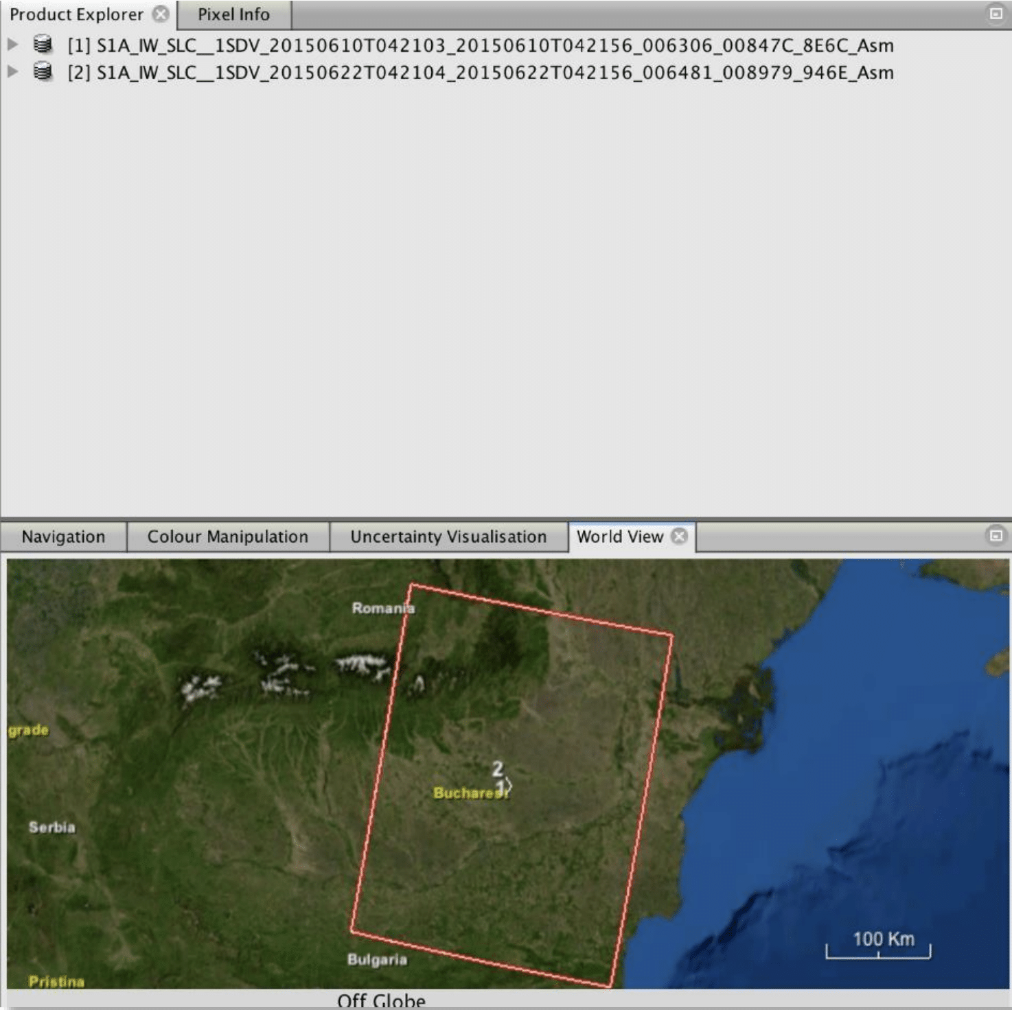
In order to create an RGB composite, the input products should be two or more SLC products over the same area acquired at different times, such as the sample images provided in this data recipe.
Open the products
Use the Open Product button in the top toolbar and browse for the location of the Sentinel-1 Interferometric Wide (IW) SLC products. To start, we will be working with both images from 6/10/2015, as seen in the filename.
Note: Do NOT unzip the download files.
Press and hold the Ctrl button on your keyboard and select the files. Click Open to load the files into the toolbox.
View the products
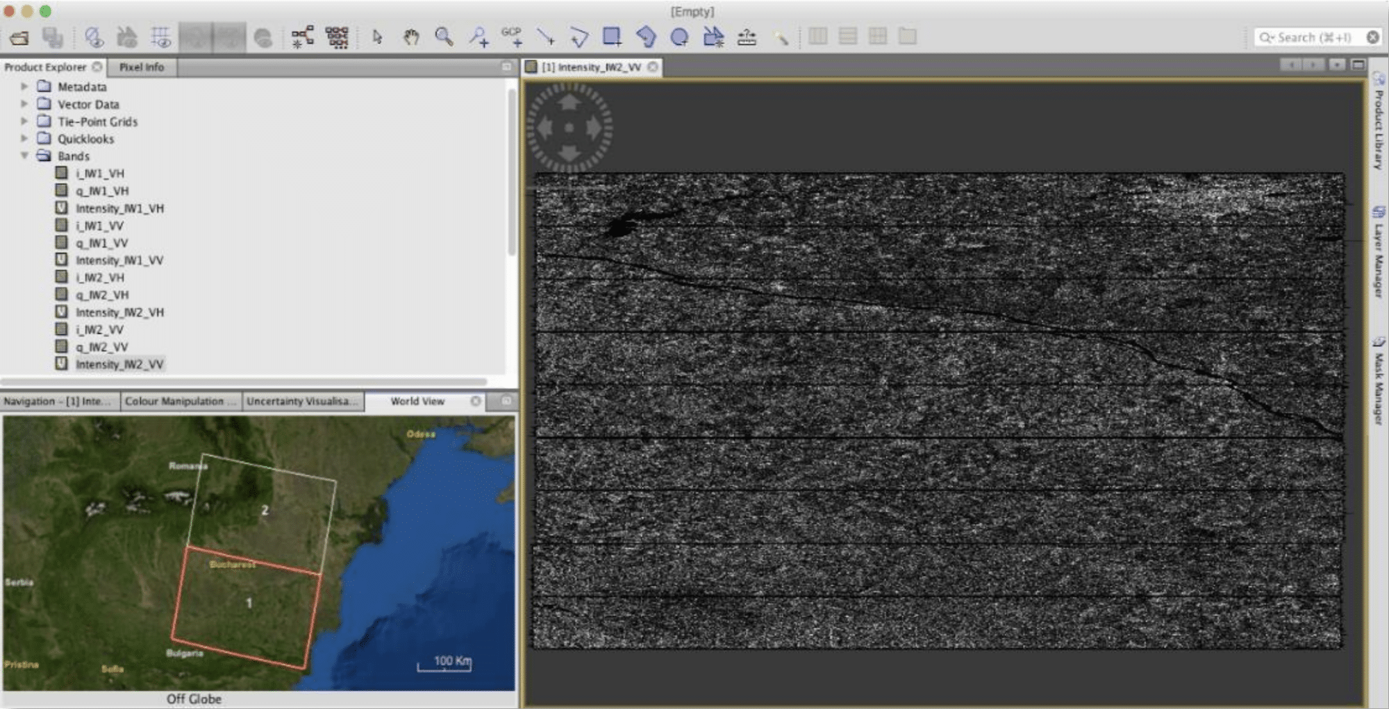
- In the Product Explorer window, you will find the products
- Double-click on each product to expand the view
- Double-click Bands to expand the folder
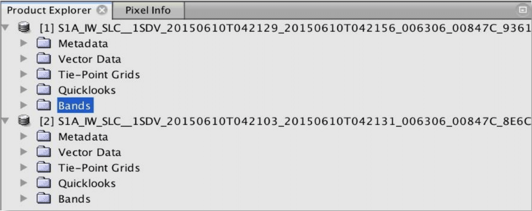
In the Bands folder, you will find bands containing the real (i) and imaginary (q) parts of the complex data. The i and q bands are the bands that are actually in the product and represent amplitude and phase. The Virtual Intesity or V-band is there to assist you in working with and visualizing the complex data.
Note that in Sentinel-1 IW SLC products, you will find three subswaths labeled IW1, IW2, and IW3. Each subswath is for an adjacent acquisition by the TOPS mode.
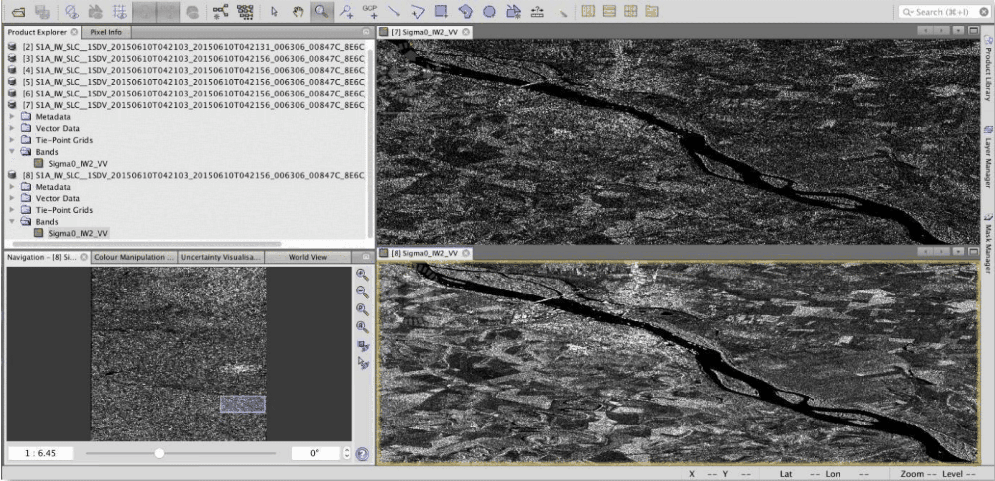
View a band
To view the data, double-click on the Intensity_IW2_VV band of one of the images. Zoom-in on the image and pan by using the tools in the Navigation window below the Product Explorer window.
Within a subswath, TOPS data are acquired in bursts. Each burst is separated by a demarcation zone. Any “data” within these demarcation zones can be considered invalid and should be zero-filled, but may also contain garbage values.
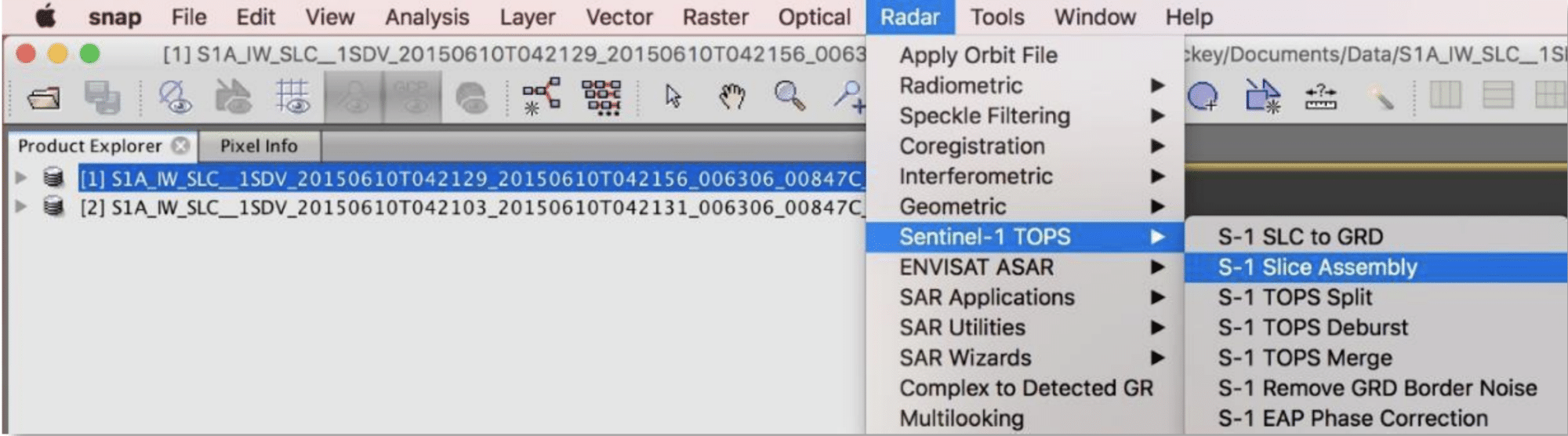
TOPS Slice Assembly
- In the top menu, navigate to Radar > Sentinel-1 TOPS > S-1 Slice Assembly
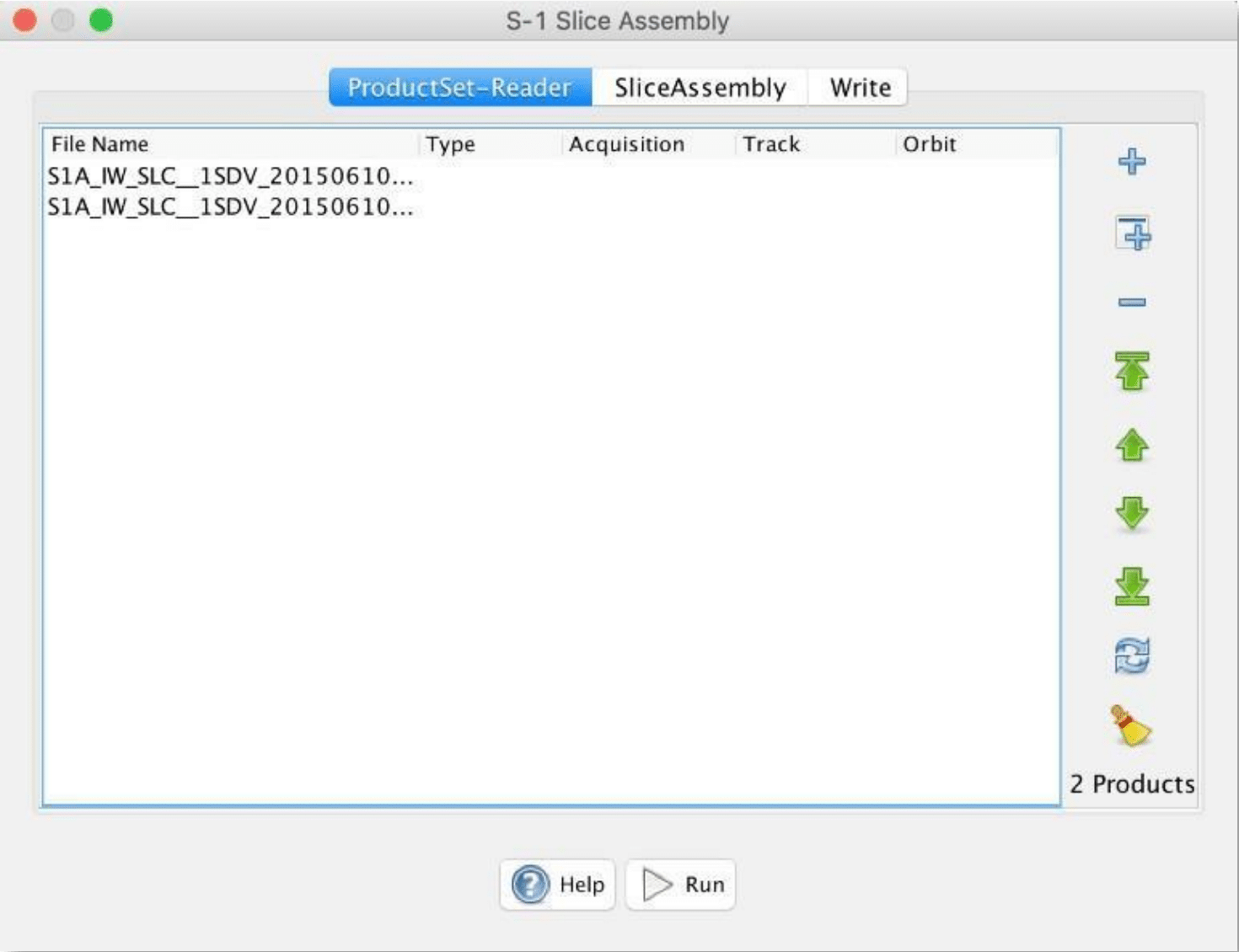
- In the ProductSet-Reader tab, add both products acquired on 06/10/2015 by using the add button (+).
- In the SliceAssembly tab, select the VV polarization
- In the Write tab, save the resulting product to a folder of your choice (e.g., 20150610_assembled)
The resulting product will automatically be appended with _Asm.
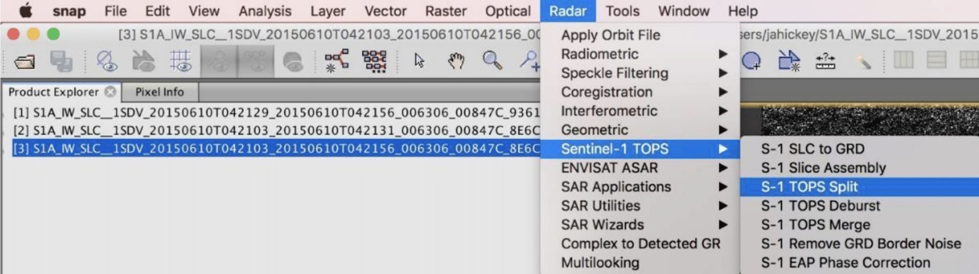
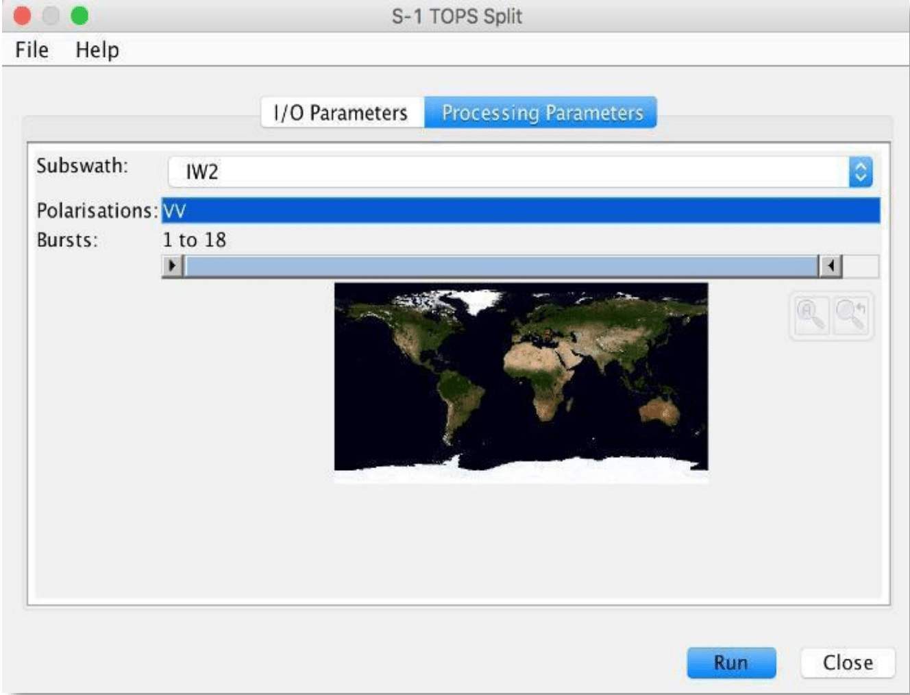
Splitting Subswaths
- In the top menu, navigate to Radar > Sentinel-1 TOPS > S-1 TOPS Split
- In I/O Parameters, for Source Product select the product from the previous step (appended with _Asm)
- In Processing Parameters, select IW2 as your Subswath
- For Polarizations, select VV
- Click Run
The resulting product will be appended with _Asm_split
Applying Precise Orbits (POD)
Orbit auxiliary data contain information about the position of the satellite during the acquisition of SAR data. Orbit data are automatically downloaded by SNAP and no manual search is required by the user.
The Precise Orbit Determination (POD) service for Sentinel-1 provides Restituted orbit files and Precise Orbit Ephemerides (POE) orbit files. POE files cover approximately 28 hours and contain orbit state vectors at fixed time steps of 10-second intervals. Files are generated one file per day and are delivered within 20 days after data acquisition. If Precise orbits are not yet available for your product, you may select the Resituted orbits, which may not be as accurate as the Precise orbits, but will be better than the predicted orbits available within the product.
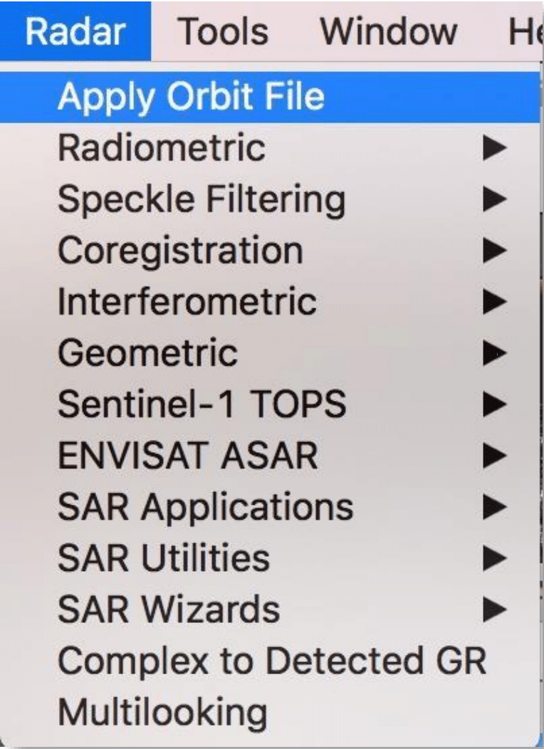
Apply Orbit File
- In the top menu, navigate to Radar > Apply Orbit File
- In the I/O Parameters, for Source Product select the product from the previous step (appended with _Asm_split)
- Click Run
The resulting product will be appended with _Asm_split_Orb
Radiometric Calibration
Radiometric calibration corrects a SAR image so that the pixel values truly represent the radar backscatter of the reflecting surface.
The corrections applied during calibration are mission-specific, therefore the software will automatically determine what kind of input product you have and what corrections need to be applied based on the product’s metadata.
Calibration is essential for quantitative use of SAR data.
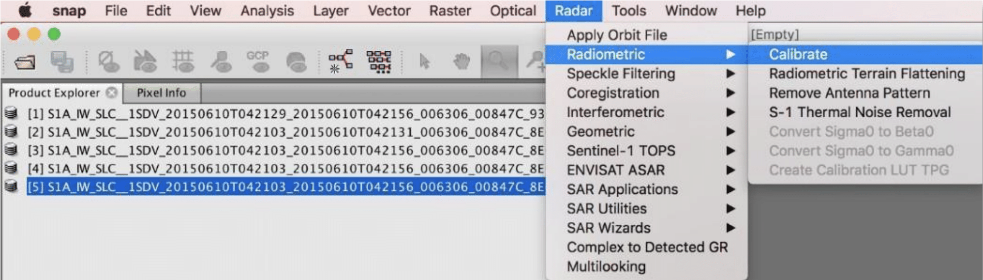
Calibrate a Sentinel-1 image
- In the top menu, navigate to Radar > Radiometric > Calibrate
- In I/O Parameters, for Source Product, select the product from the previous step (appended with _Asm_split_Orb)
- In Processing Parameters, select VV
- Select Output sigma0 band
- Click Run
The resulting product will be appended with _Asm_split_Orb_Cal

TOPS Debursting
To seamlessly join all burst data into a single image, apply the TOPS Deburst operator from the Sentinel-1 TOPS menu.
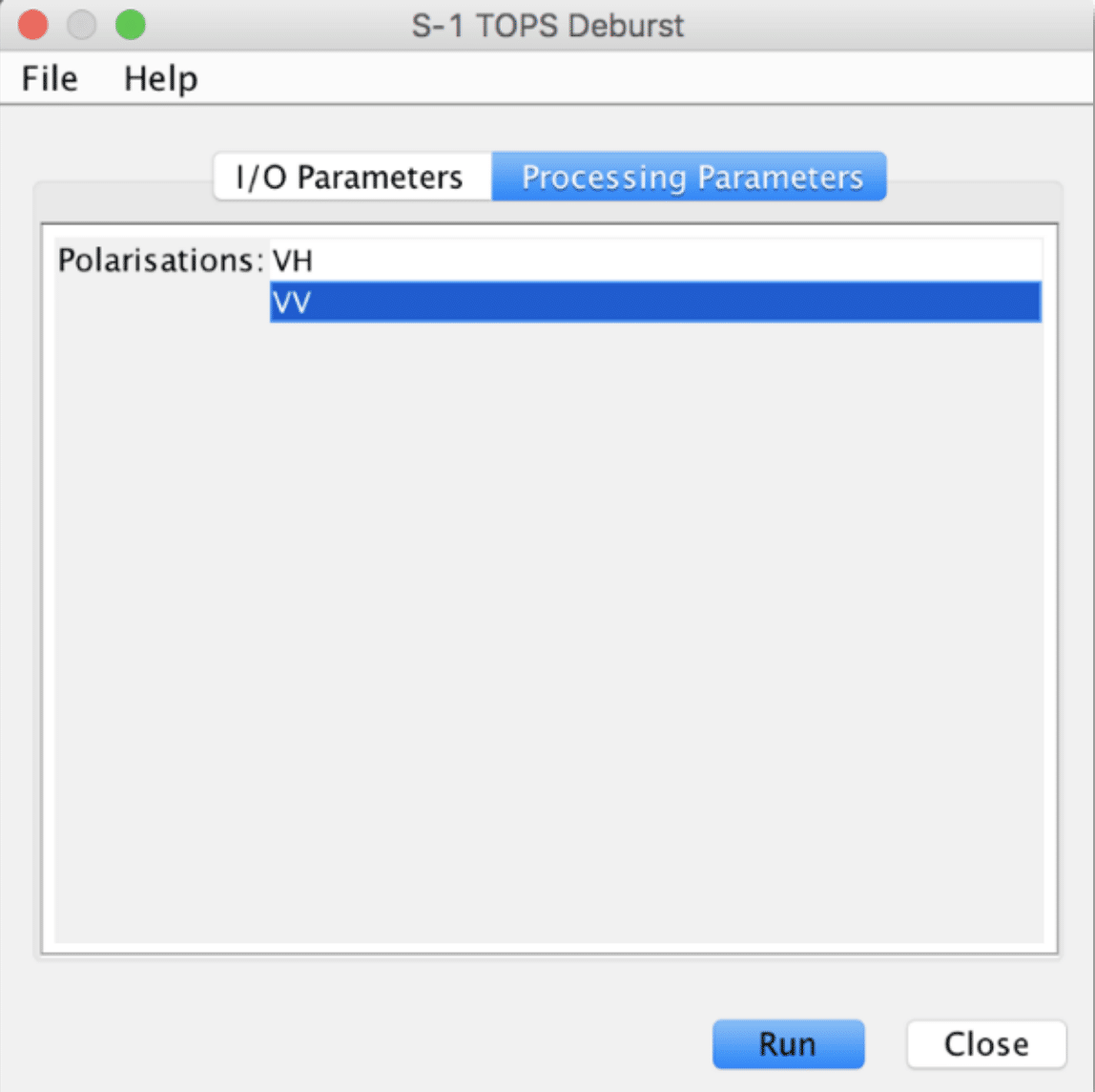
Deburst Image
- In the top menu, navigate to Radar > Sentinel-1 > S-1 TOPS Deburst
- In I/O Parameters, for Source Product, select the product from the previous step (appended with _Asm_split_Orb_Cal)
- In Processing Parameters, Select VV
- Click Run
The resulting product will be appended with _Asm_split_Orb_Cal_deb

Speckle Reduction
Speckle is caused by random constructive and destructive interference resulting in salt and pepper noise throughout the image. Speckle filters can be applied to the data to reduce the amount of speckle at the cost of blurred features or reduced resolution.
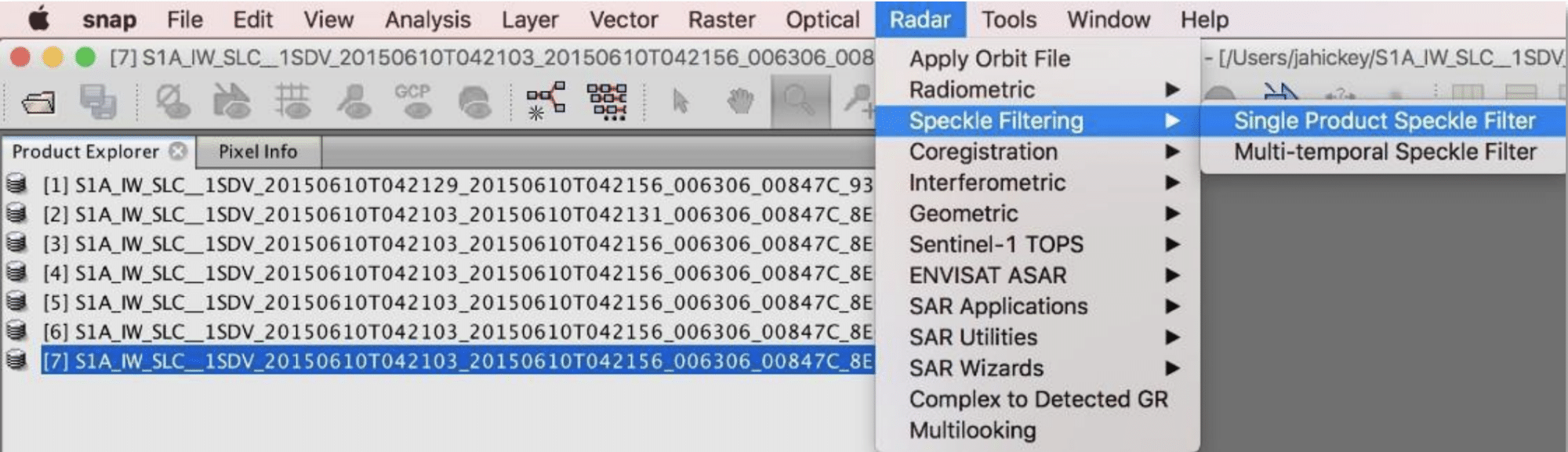
Speckle Filtering
- In the top menu, navigate to Radar > Speckle Filtering > Single Product Speckle Filter
- In I/O Parameters, for Source Product, select the product from the previous step (appended with _Asm_split_Orb_Cal_deb)
- In Processing Parameters, set Filter to Gamma Map
- The Gamma Map filter assumes that the scene reflectivity of an image has a Gaussian distribution. Therefore, this filter uses a priori knowledge of the probability density function (PDF) of the scene when suppressing the speckle of the image.
- Click Run
The resulting product will be appended with _Asm_split_Orb_Cal_deb_Spk
SAR Multi-looking
Multi-look processing can be used to produce a product with nominal image pixel size.
Multiple looks may be generated by averaging over range and/or azimuth resolution cells improving radiometric resolution but degrading spatial resolution. As a result, the image will have less noise and approximate square pixel spacing after being converted from slant range to ground range.
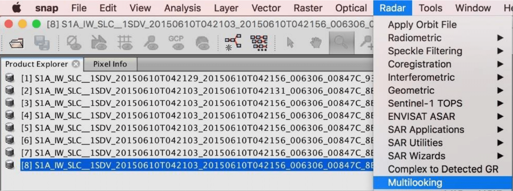
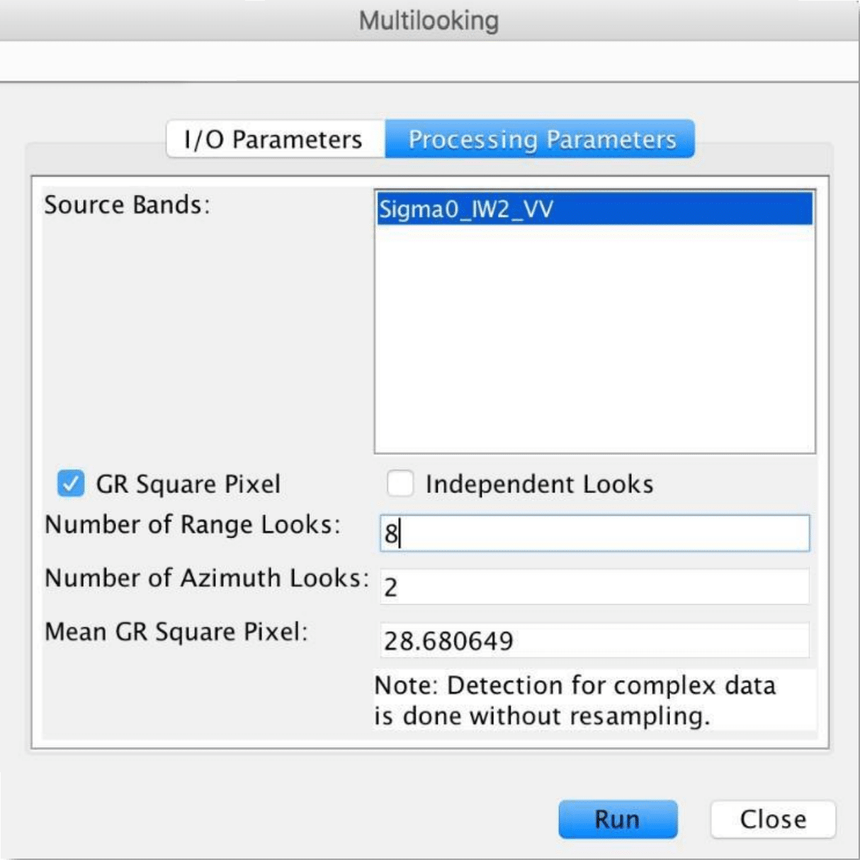
Multi-look the image
- In the top menu, navigate to Radar > Multilooking
- In I/O Parameters, for Source Product select the product from the previous step (appended with _Asm_split_Orb_Cal_deb_Spk)
- In the Processing Parameters tab, change Number of Range Looks to 8. Notice that the Number of Azimuth Looks automatically changes to 2.
- Click Run
The resulting product will be appended with _Asm_split_Orb_Cal_deb_Spk_ML
Note: You must now repeat the steps in Part 1: Processing SLC Image Pairs for the second pair of images acquired on 06/22/2015.
Remove all products from the Product Explorer window by selecting the products, then right-click and choose Close All Products.
Part 2: TOPS Coregistration and InSAR Coherence
Open Assembled SLC Images
In order to create the bands necessary for the RGB composite image, you will have to co-register the images created in Part 1: Processing SLC Image Pairs — TOPS Slice Assembly. These assembled SLC products will allow you to estimate the coherence between the two images.
Open the products
Use the Open Product button in the top toolbar and browse to the location of the assembled SLC products. These images will have the suffix _asm.dim (if you did not choose to create a custom file name).
S-1 TOPS Coregistration
For Interferometric processing (coherence estimation), two or more images must be coregistered into a stack. One image is selected as the master and the other images are the “slaves.” The pixels in the “slave” images will be moved to align with the master image to sub-pixel accuracy.
Coregistration ensures that each ground target contributes to the same (range, azimuth) pixel in both the master and the “slave” image. For TOPSAR InSAR, S-1 TOPS Coregistration is used.
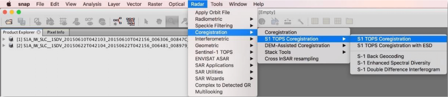
Coregister the images
Navigate to Radar > Coregistration > S1 TOPS Coregistration > S1 TOPS Coregistration
- In the Read tab, select the first product — this will be your master image
- In the Read(2) tab, select the other product — this will be your “slave” image
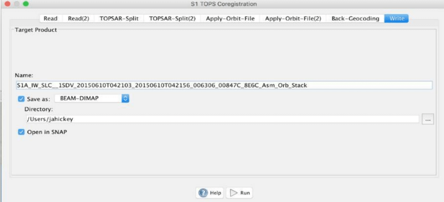
- In the TOPSAR-Split tabs, select the IW2 subswath for each of the products
- In the Apply-Orbit-File tabs, select the Sentinel Precise Orbit State Vectors
- In the Back-Geocoding tab, leave all parameters to default
- In the Write tab, set the Directory path to your working directory
- Click Run to begin co-registering the data
The resulting coregistered stack product will appear in the Product Explorer window with the suffix _Asm_Orb_Stack
InSAR Coherence Estimation
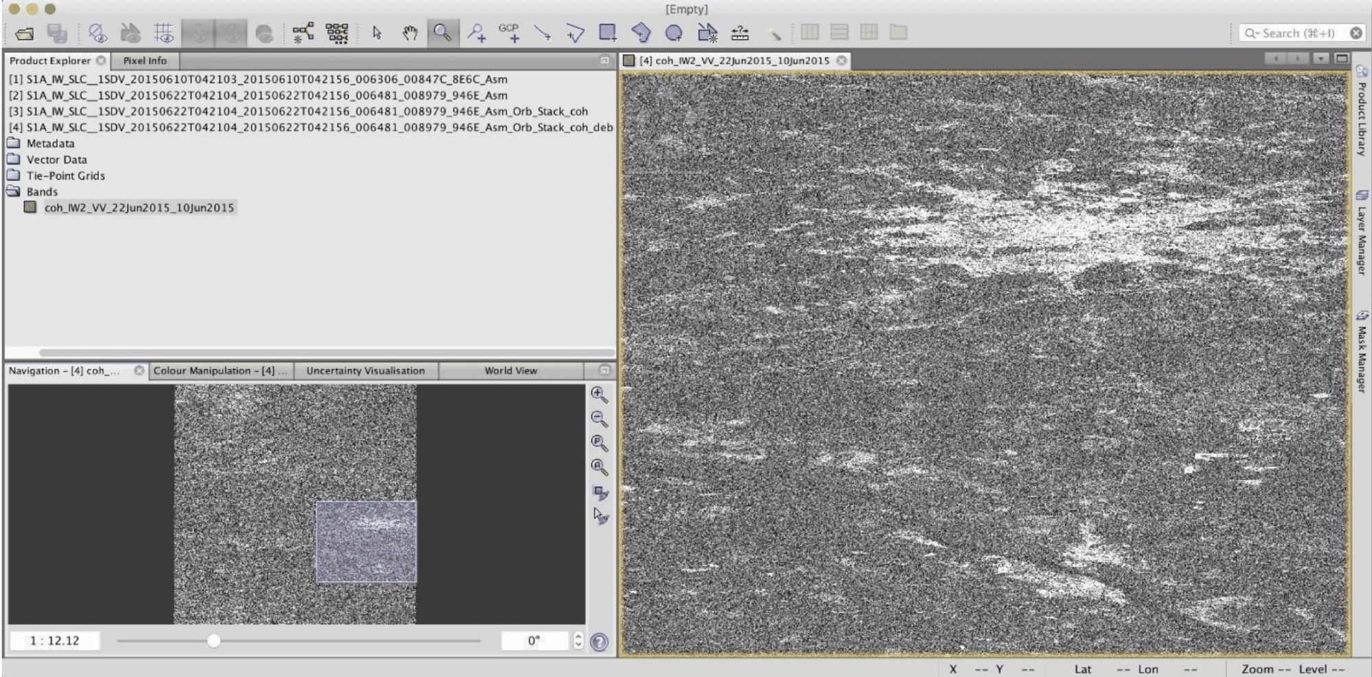
The coherence band shows how similar each pixel is between the slave and master images on a scale of 0 to 1. Areas of high coherence will appear bright. Areas with poor coherence will be dark.
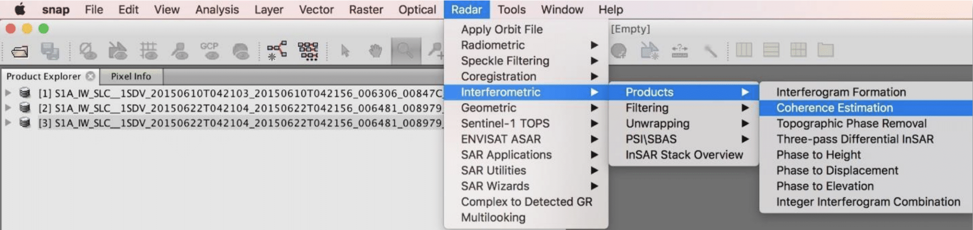
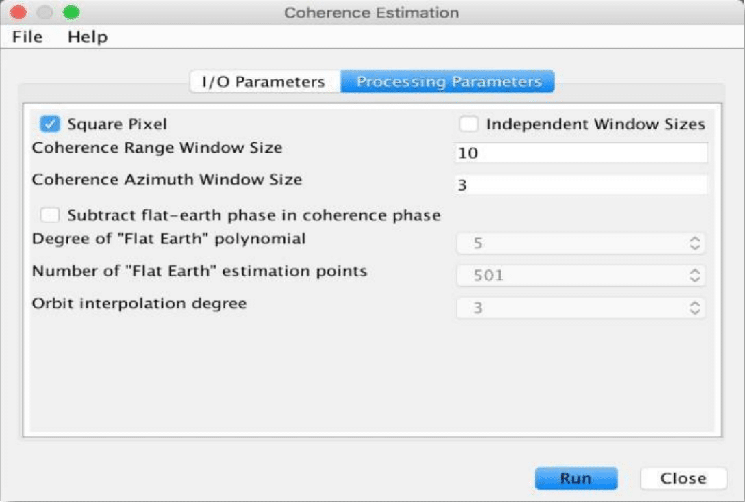
Coherence Estimation
- In the top menu, navigate to Radar > Interferometric > Products > Coherence Estimation
- In I/O Parameters, for Source Product select the product from the previous step (appended with _Asm_Orb_Stack)
- Click Run
The resulting product will be appended with _Asm_Orb_Stack_coh

TOPS Debursting
- In the top menu, navigate to Radar > Sentinel-1 TOPS > S-1 TOPS Deburst
- In I/O Parameters, for Source Product, select the product from the previous step (appended with _Asm_Orb_Stack_coh)
- Click Run
The resulting product will be appended with _Asm_Orb_Stack_coh_deb

Multilooking
- In the top menu, navigate to Radar > Multilooking
- In I/O Parameters, for Source Product, select the product from the previous step (appended _Asm_Orb_Stack_coh_deb)
- In the Processing Parameters tab, change the Number of Range Looks to 8; the Number of Azimuth Looks automatically changes to 2.
- Click Run
The resulting product will be appended with _Asm_Orb_Stack_coh_deb_ML
Note: Before proceeding with Generating an RGB Composite, remove all products from the Product Explorer window except for the final, multi-looked product (ending with _ML). Left-click on the _ML product to highlight it, then from the top menu select File > Close Other Products.
Part 3: Generating an RGB Composite
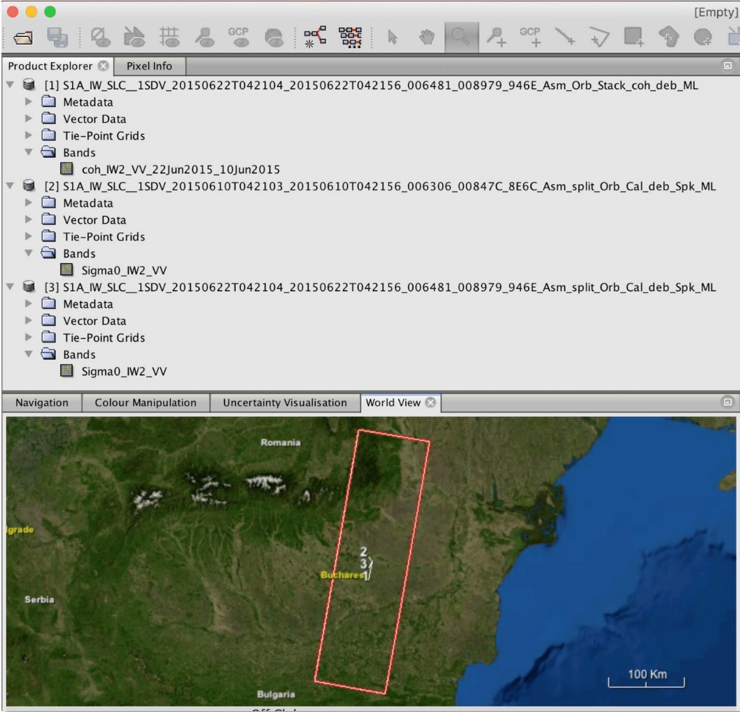
Open Processed Images, Coherence Stack
For this part, we will use the final two products we created in Part 1: Processing SLC Image Pairs (appended with _ML) and the final product in Part 2: TOPS Coregistration and InSAR Coherence (also appended with _ML) to generate our complex Sentinel-1 TOPS RGB composite.
Open Final Products
Navigate to the folder you chose to store the products created in Processing SLC Image Pairs and TOPS Coregistration and InSAR Coherence. Open the products with the filename ending in _ML.dim.
- Use the Open Product button to add the products into the Product Explorer
- You may view the products by double-clicking on each item and expanding the Bands folder
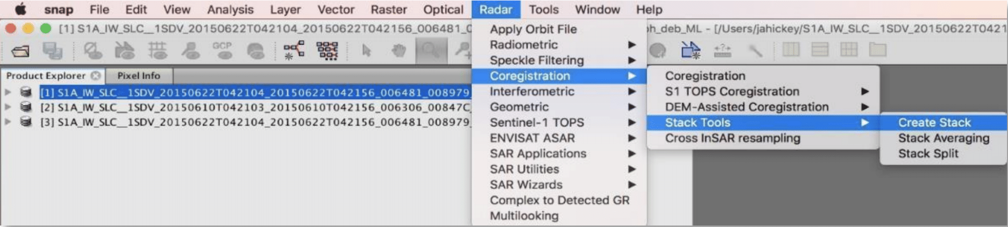
Create Data Stack
Creating a data stack will tie each of your final products together and create a single product with multiple bands. Each band will represent the single band present in each of your products. We will use these three bands to generate our composite image.
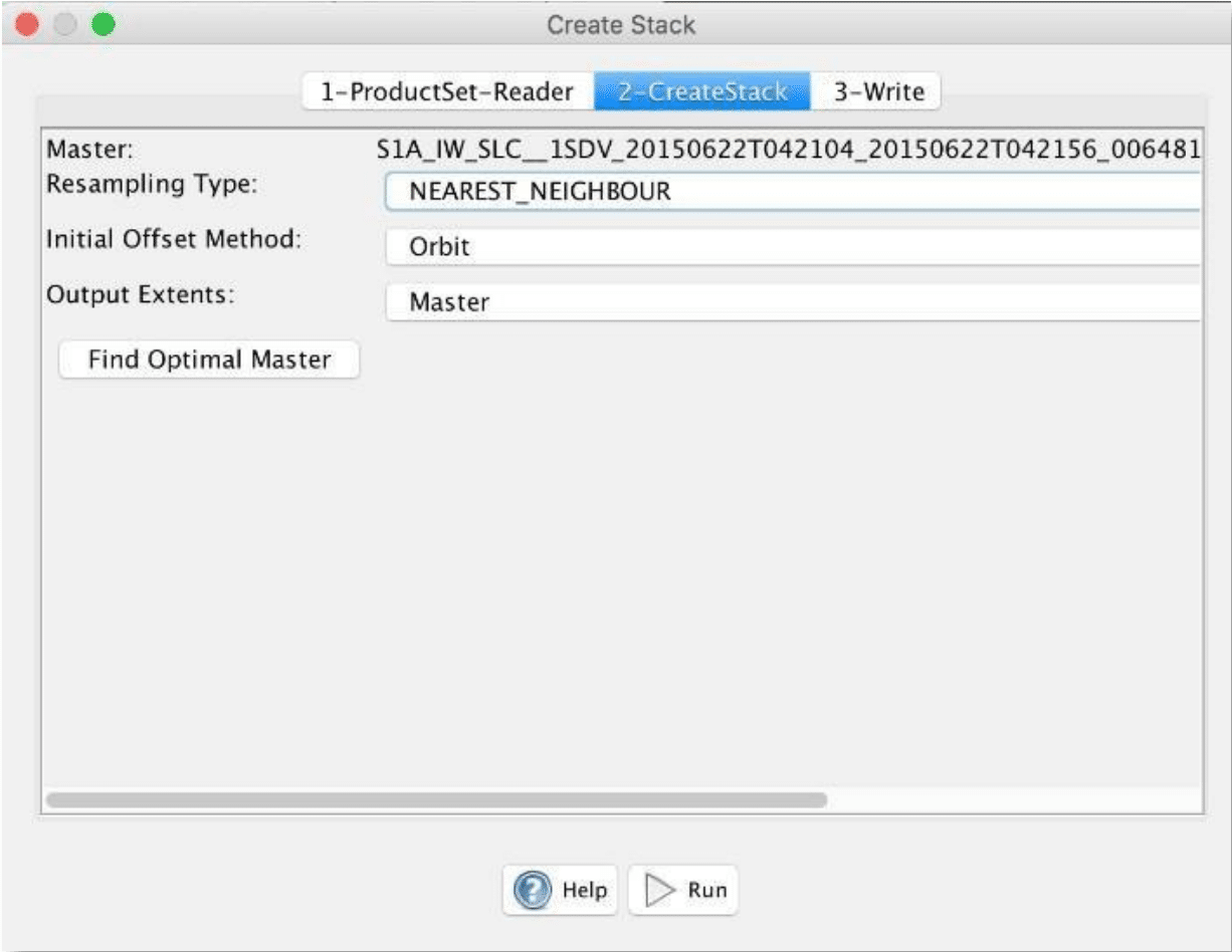
Create Stack
- Navigate to Radar > Coregistration > Stack Tools > Create Stack
- In Create Stack, add the three products to the ProductSet-Reader by clicking on the Add Opened button (the second + sign on the right)
- In the CreateStack tab, set the Resampling Type to NEAREST NEIGHBOUR
- In the Write tab, set the directory to store the product
- Click Run
Your product will appear in the Product Explorer and will have all three bands.
Create Spatial Subset over your Area of Interest
In this particular example, our area of interest will be the capital of Romania, Bucharest, and the surrounding area. This step is not necessary but is useful if you are only interested in a particular region and desire to crop the image.
Create Subset
- Double-click on the opened product to view the product bands
- Double-click on any of the bands inside the product
- Zoom in using the mouse wheel and dragging the left mouse button
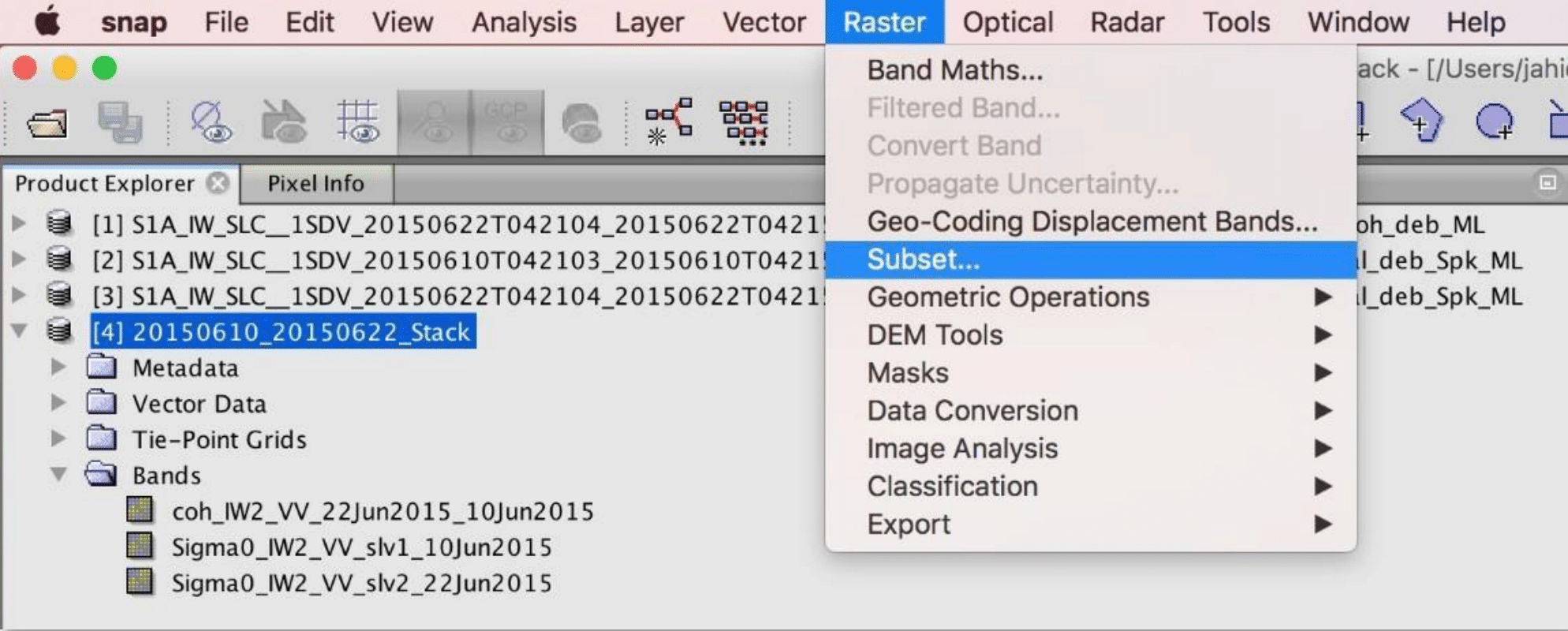
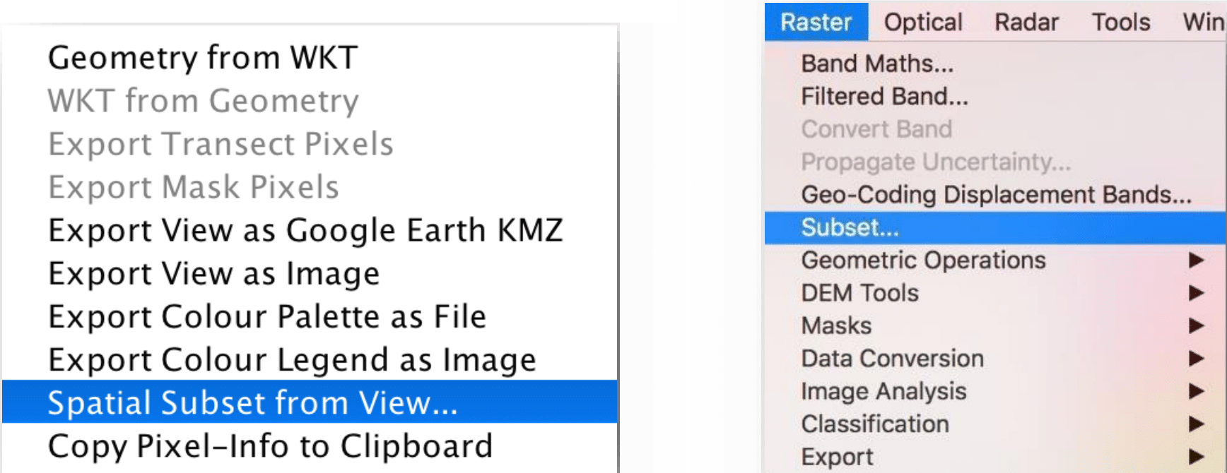
- Once you have zoomed and panned to your area of interest, right-click and select Spatial Subset from View in the context menu.
- You may also access this option via the Raster menu by selecting Subset…
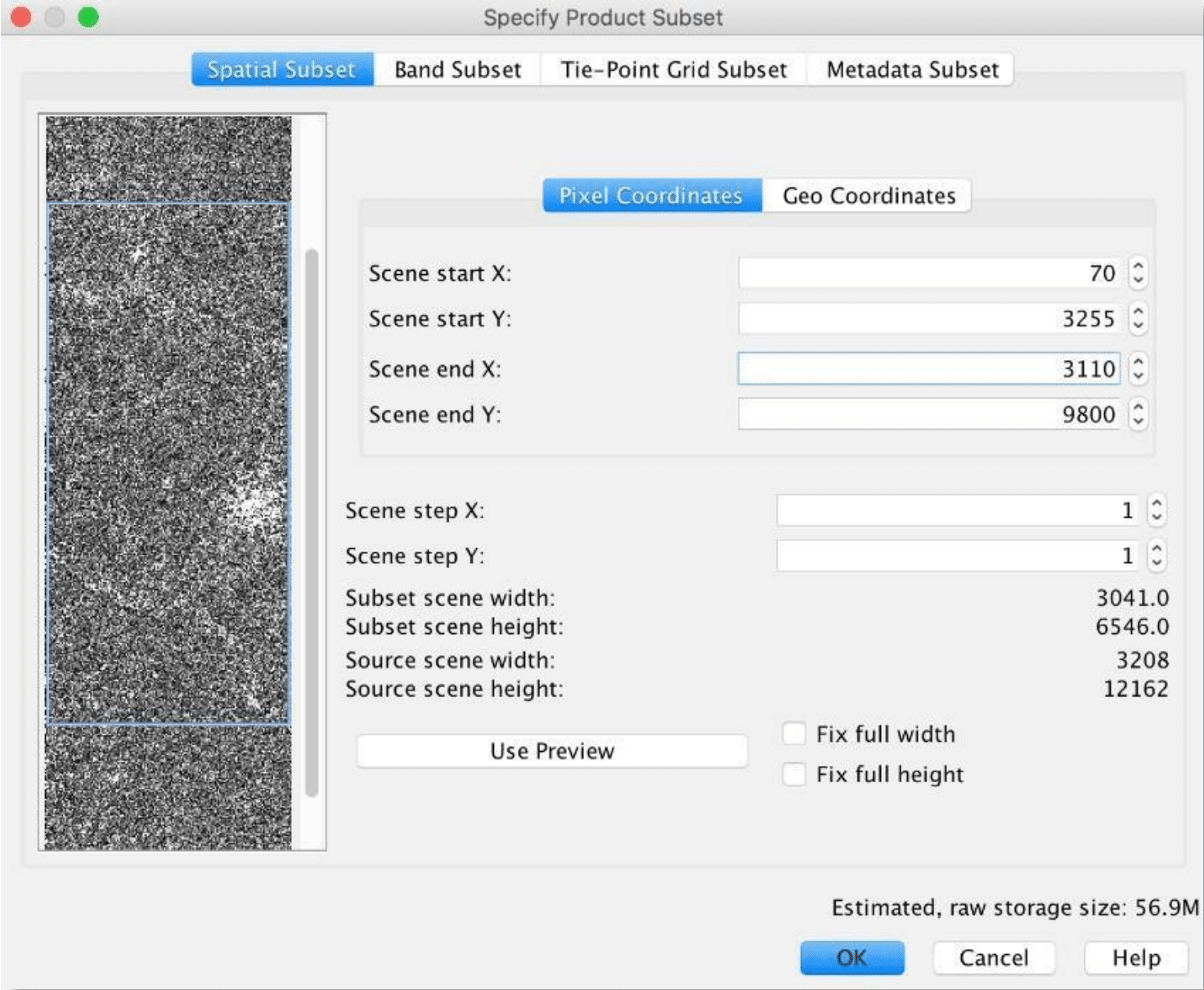
The subset dialog box will automatically select the area you were viewing. To adjust the extent of your subset image, you may drag the bounding box, enter the pixel coordinates, or add geo-coordinates.
Click OK to create your subset image.
When the new subset product appears in the Product Explorer:
- Right-click on the product
- Select Save Product in the context menu
- Select Yes to convert the product to the BEAM-DIMAP format
Range-Doppler Terrain Correction
Terrain Correction will geocode the image by correcting SAR geometric distortions using a digital elevation model (DEM) and producing a map-projected product.
Geocoding converts an image from Slant Range, or Ground Range, Geometry into a Map Coordinate System. Terrain Geocoding involves using a DEM to correct inherent geometry effects such as foreshortening, layover and shadow
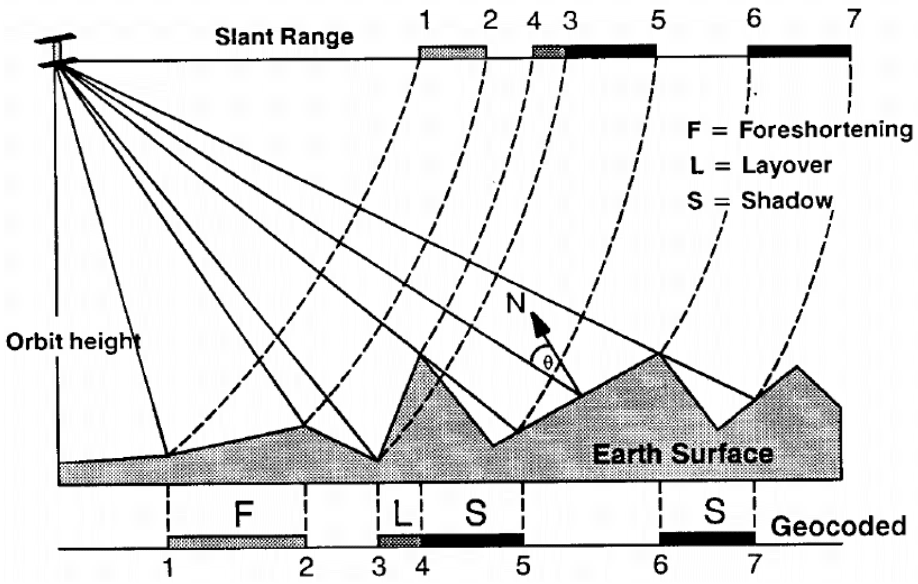
Foreshortening
- The period of time a slope is illuminated by the transmitted pulse of the radar energy determines the length of the slope on radar imagery.
- This results in shortening of a terrain slope on radar imagery in all cases except when the local angle of incidence ( ) is equal to 90° ( ).
Layover
- When the top of the terrain slope is closer to the radar platform than the bottom, the former will be recorded sooner than the latter.
- The sequence at which the points along the terrain are imaged produces an image that appears inverted.
- Radar layover is dependent on the difference in slant range distance between the top and bottom of the feature.
Shadow
- The back-slope is obscured from the imaging beam causing to return no area of radar shadow.
The effects of these distortions can be seen in the Slant Range image. The distance between 1 and 2 can appear shorter than it should and the return for 4 can occur before the return for 3 due to the elevation.
Terrain Correction
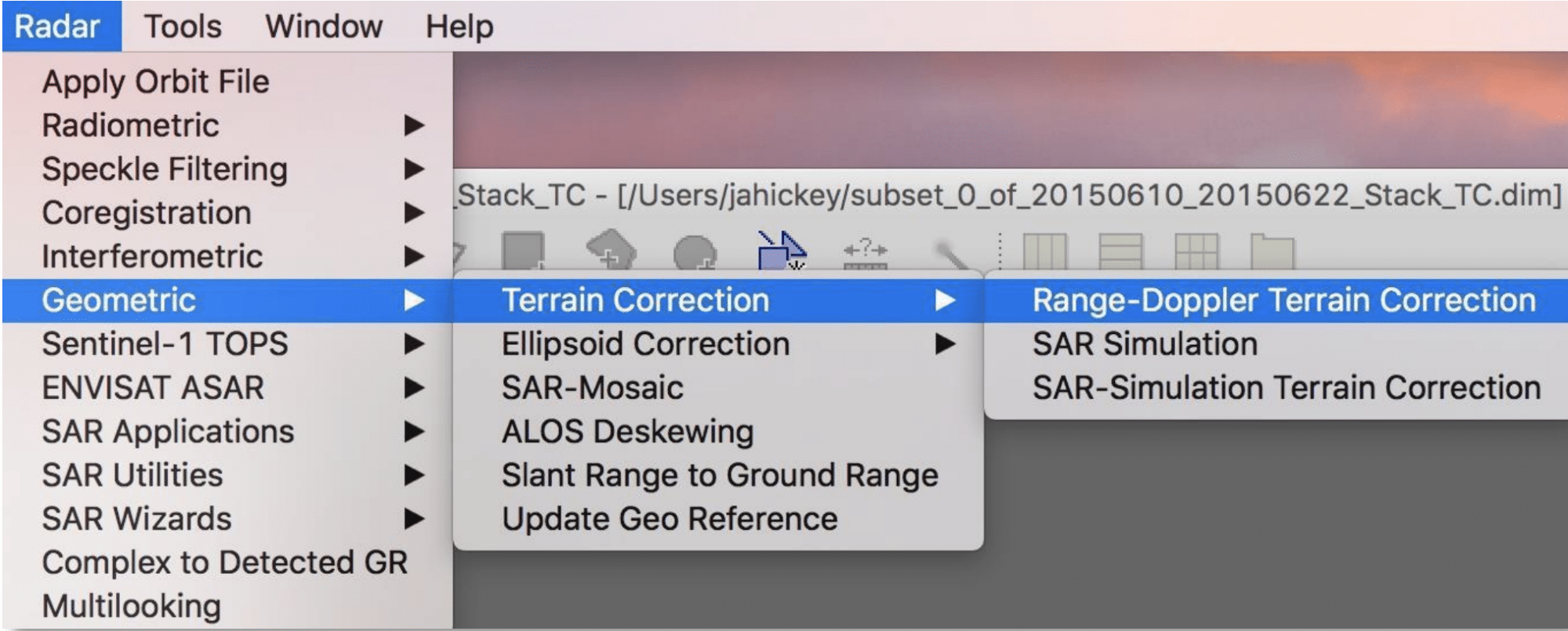
- Highlight the subset product in Product Explorer
- In the top menu, navigate to Radar > Geometric > Terrain Correction > Range-Doppler Terrain Correction
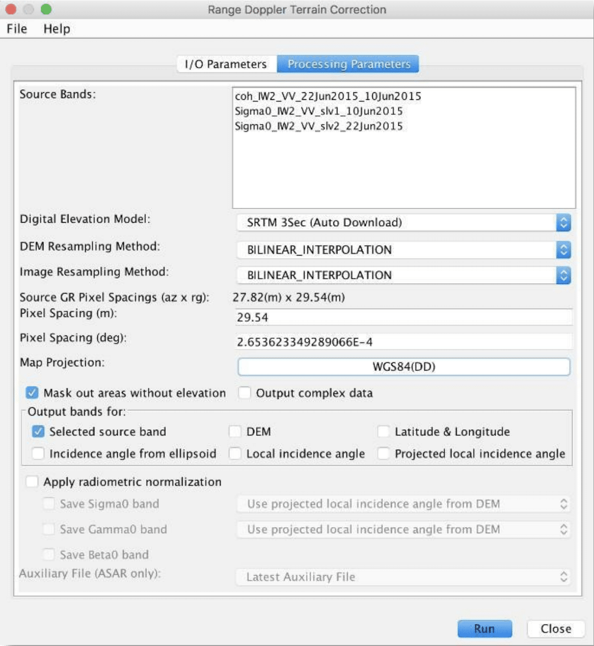
- By default, the terrain correction will use the SRTM 3 sec DEM. The software will automatically determine the DEM tiles needed and download them from internet servers
- In Processing Parameters, leave all parameters as default
Note: You may choose a projection of your liking, however, you will not be able to export to Google Earth unless you have Lat/Long coordinates
- Click Run
Band Math Tool
This step will allow us to create meaningful bands used in our composite RGB image. This is a three-step process and will create several virtual bands.
Create Average Backscatter Band
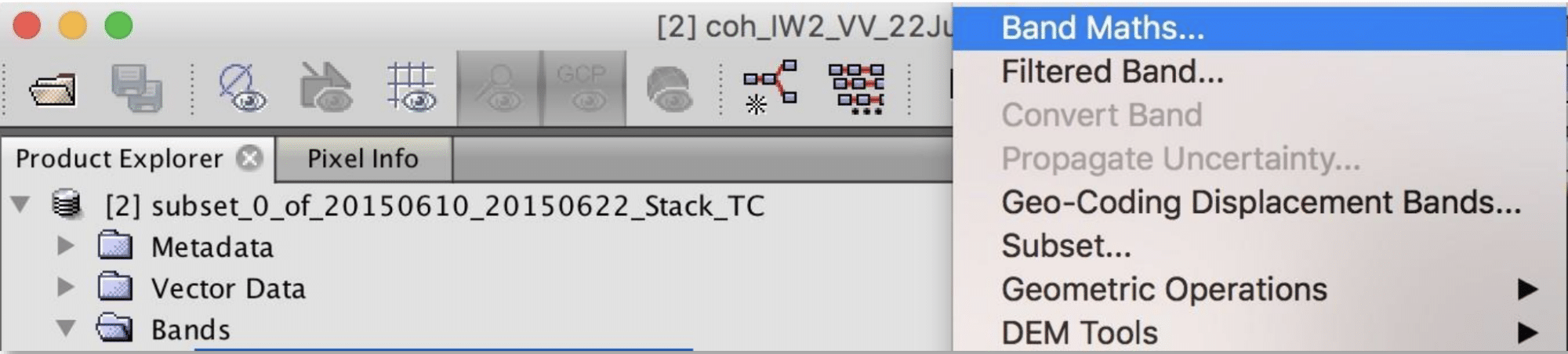
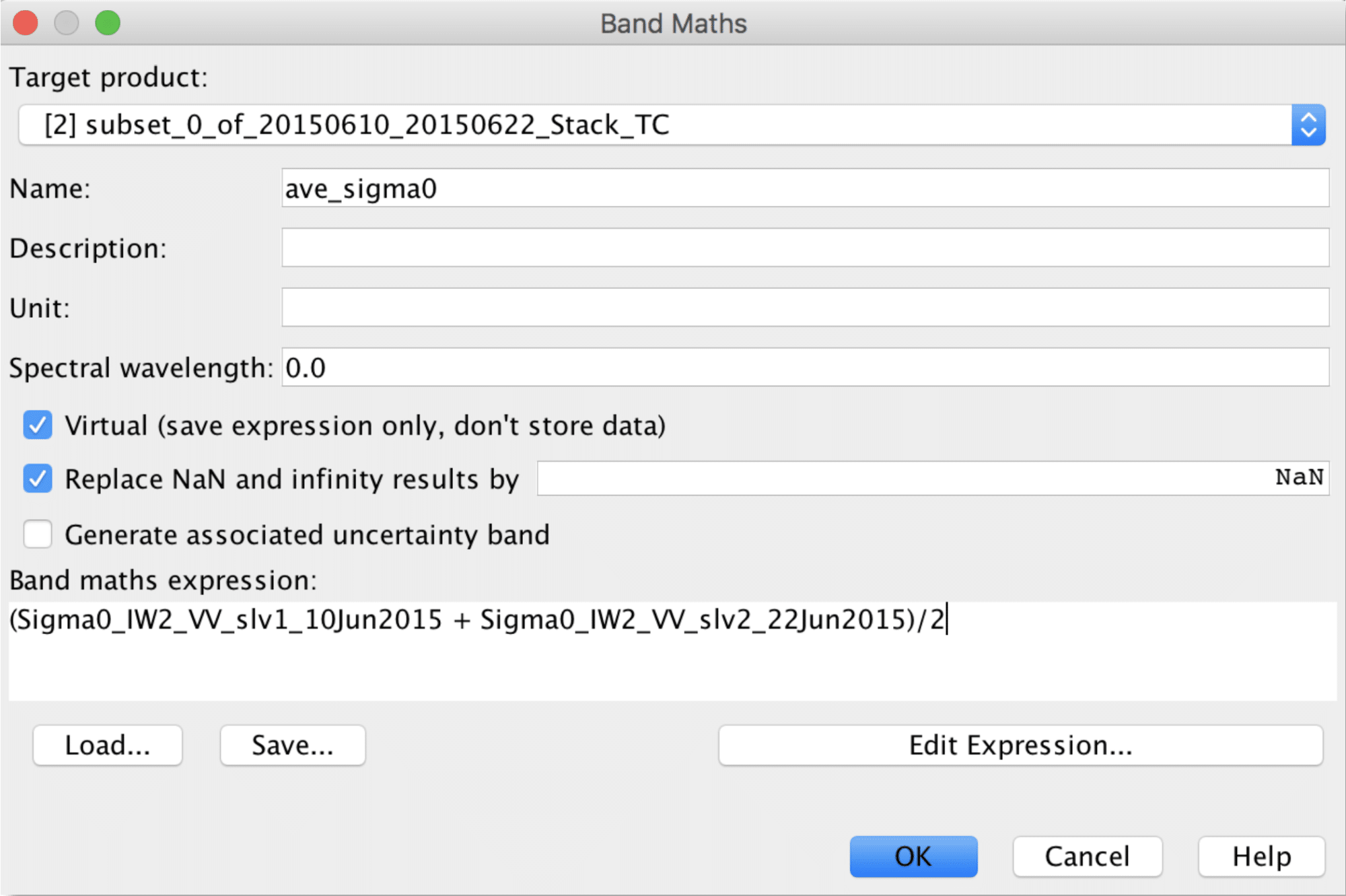
- In the top menu, navigate to Raster > Band Maths
- In the Band Maths window:
- Select the terrain-corrected subset product (_TC)
- Name the band ave_sigma0
- Click on the Edit Expression… button
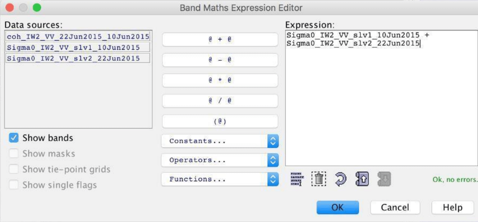
- In the Band Maths Expression Editor:
- Click the @ + @ operator
- Click on the two Sigma0 products in Data sources and they will be added to the expression
- Click OK
- In the Band Maths Expression box:
- Add parenthesis around the expression and type /2 (divided by 2)
The expression should look like: (Sigma0_6-22-2015 + Sigma0_06-10-2015)/2
- Click OK to create the virtual band
Create Backscatter Difference Band
- In the top menu, navigate to Raster > Band Maths
- In the Band Maths window:
- Select the terrain-corrected subset product (_TC)
- Name the band diff_sigma0
- Open the Band Maths Expression Editor by clicking the Edit Expression… button
- In the Band Maths Expression Editor:
- Delete the contents of the Expression: box
- Click the @ – @ operator
- Click on the two Sigma0 products in Data sources and they will be added to the expression
- Click OK
Your final expression should look like this: older Sigma0 – newer Sigma0
- Click OK to create the virtual band
Linear to dB Scale Conversion
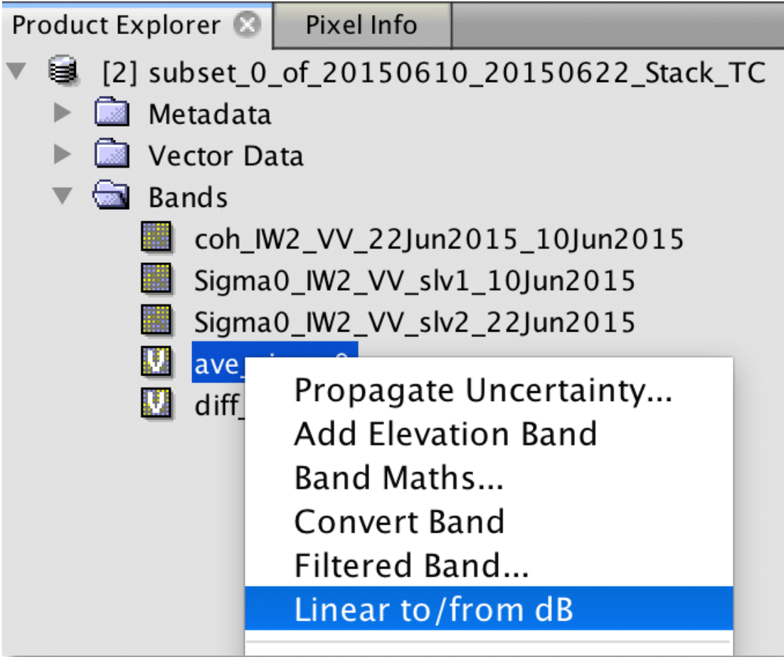
- Double-click on the terrain-corrected subset product (_TC) in Product Explorer
- Open the Bands folder
- Right-click on the band named ave_sigma0
- Click Linear to/from dB
- When prompted, click Yes to create a new virtual band
Note: You may also find this function in Raster > Data Conversion > Linear to/from dB
Optional — Save Virtual Bands
To permanently save the virtual bands within your product file:
- In the Product Explorer, right-click on the newly-created virtual bands (e.g., ave_sig0)
- From the context menu, select Convert Band
RGB Composite Generation
Open the RGB Image
- Right-click on the terrain-corrected subset product (_TC) in Product Explorer
- Select Open RGB Image Window
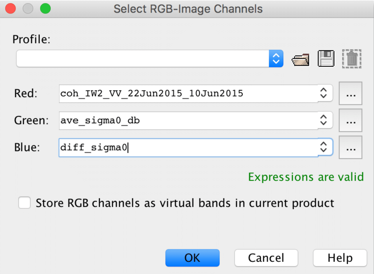
In the Select RGB-Image Channels window:
- Click on the … button next to Red
- Delete the contents of the Expression: box
- In Edit Red Expression, click the coherence product (coh_) in Data sources
- Click OK
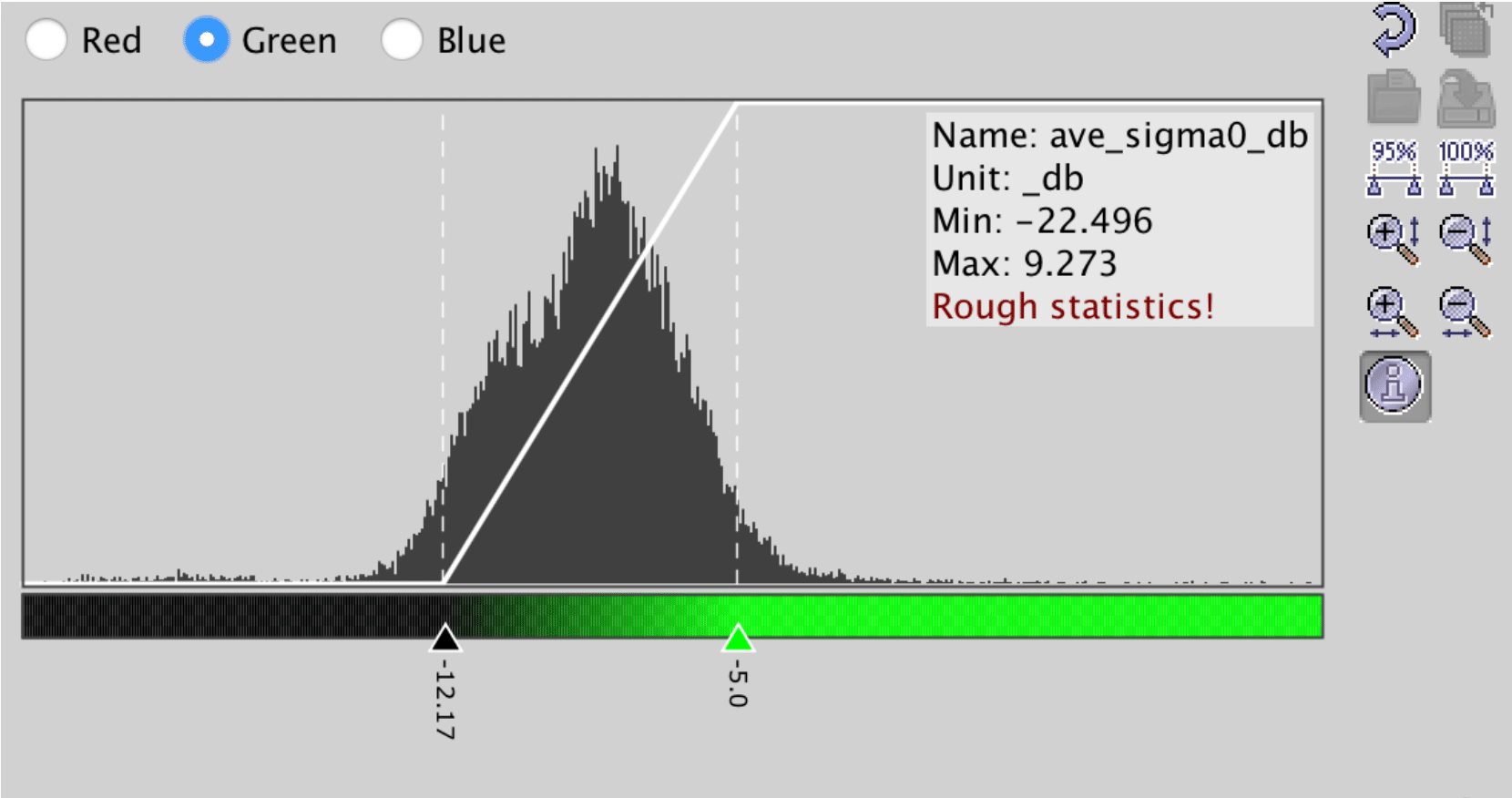
- Repeat for Green and select ave_sigma0_dB
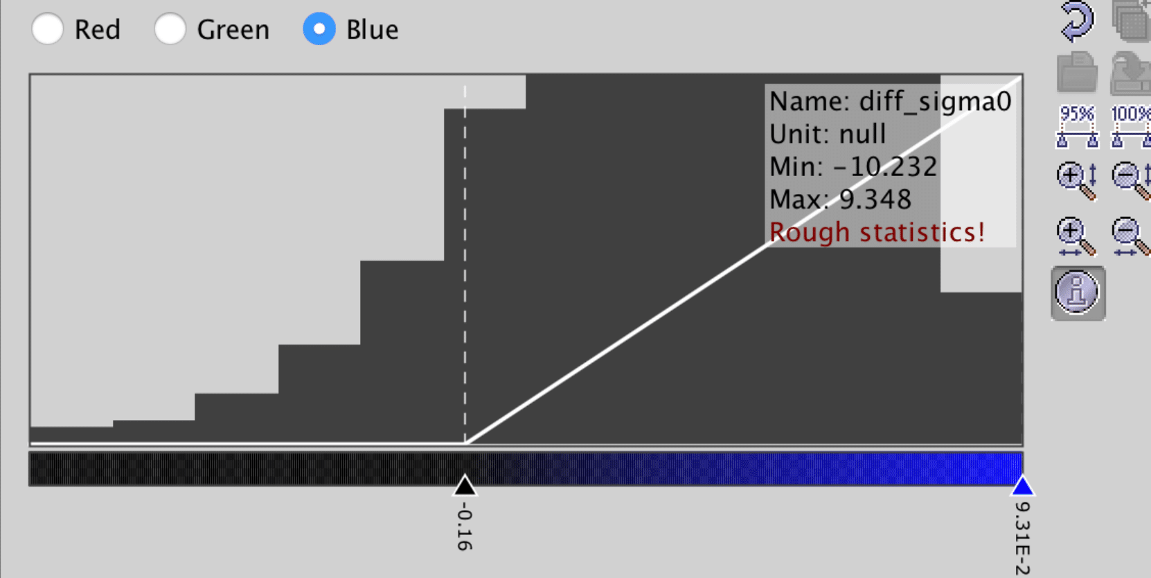
- Repeat for Blue and select diff_sigma0
- Optional — Check Store RGB channels as virtual bands in current product
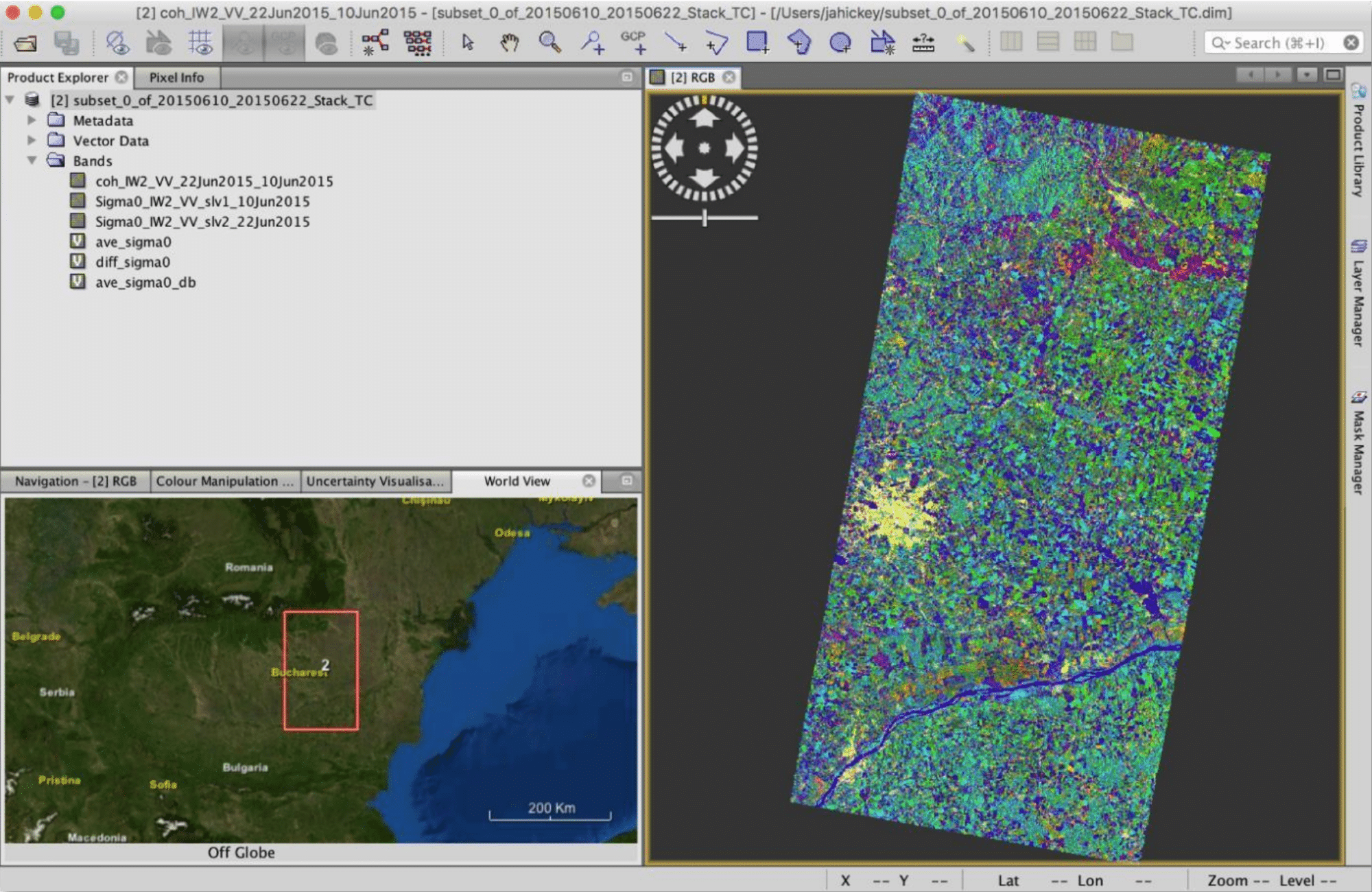
- Click OK to see results.

The resulting image may seem a little too light. To adjust color settings, click on the Color Manipulation tab below Product Explorer, or from the top menu, View > Tool Windows > Color Manipulation. The following values are suggested for each band rendering but can be adjusted to meet your needs.

Export to Google Earth
In the top menu, navigate to File > Export > Other > View as Google Earth KMZ
In addition to GeoTIFF and HDF5 formats, KMZ and various specialty formats are supported. The resulting image shows a KMZ-formatted RGB composite image overlaid on Google Earth.
The resulting image also works in a GIS environment because it is geocoded.
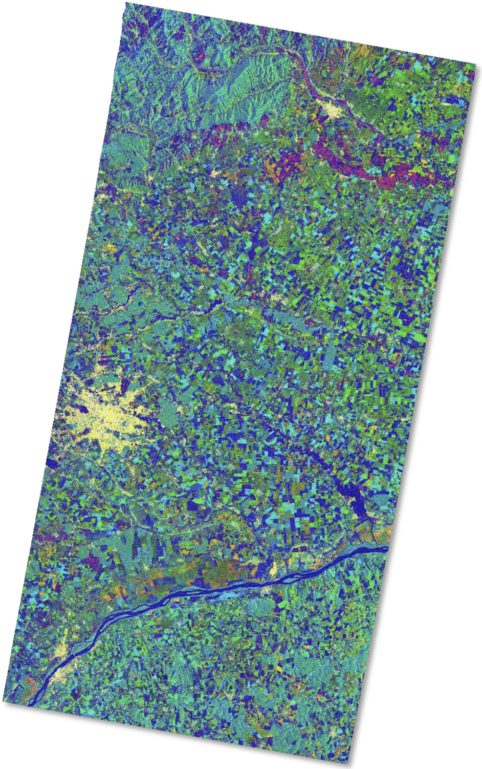
Resulting Image
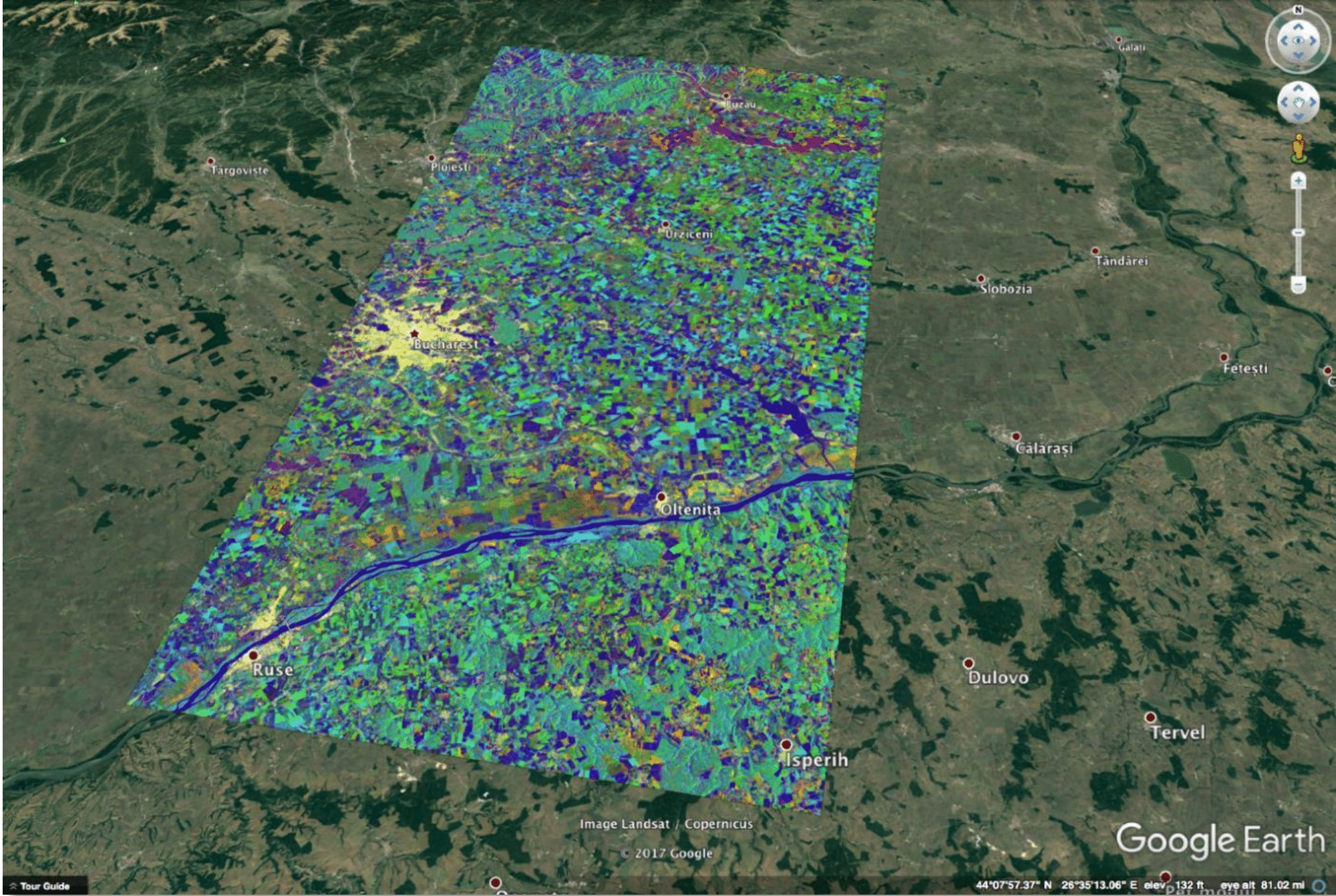
Multi-temporal color composite images give us an idea of an area’s land cover and use. Different colors show changes that occurred over the period of coverage.
The blues across the entire image represent strong changes in bodies of water or agricultural activities such as ploughing. The yellows represent urban centers, with the capital city of Bucharest very distinct. Vegetated fields and forests appear in green. The reds and oranges represent unchanging features such as bare soil or possibly rocks that border the forests.
In this data recipe, a 12-day repeat interval is used, as we are using only Sentinel-1A data. With the launch of Sentinel-1B in early 2016, this repeat cycle is reduced to 6 days, as the satellites share the same orbit. C-band coherence is significantly lower over the image after 12 days (Sentinel-1A) as compared to 6 days, which makes it more ideal to separate agricultural areas and forest, which is ideal for temperate regions.